Modeling Interactions Data with Boosted Trees

Case Study Key

Author

LASER Institute

Published

July 13, 2025

1. PREPARE

After interpreting our last model, it is easy to think we can do a little better. But, how? In this module, we’ll do do things: 1) specify a more sophisticated model and 2) go deeper on some feature engineering.

Our driving question for this module, then, is: How much can we improve our model? Looking back to our predictive model from module 3, we can see that our accuracy was okay. Can we improve on that? Let’s dive in! First, we’ll briefly review two key concepts for the module.

A more sophisticated model

we attempt to improve our predictive performance by switching to a more complex model than the logistic regression we have been using–specifically, to a type of model that is based on decision trees – a boosted‑tree model. In short, this is one way we can improve our model’s predictions.

Boosted trees (gradient boosting) build a sequence of small “decision trees” (detailed in the conceptual overview), each one focusing on the records the previous trees struggled with. When tuned carefully (small learning rate, many trees) the ensemble can outperform other algorithms based on decision trees you may have heard of, like the random forest algorithm.

A little background (and some readings) on feature engineering

Feature engineering is a rich topic in machine learning research, including in the learning analytics and educational data mining communities.

Consider research on online learning and the work of Rodriguez et al. (2021). In this study, digital trace data, data generated through users’ interactions with digital technologies. Optionally, review this paper – specifically how they processed the “clickstream” data. As this paper illustrates, there is not one way to use such data.

Rodriguez, F., Lee, H. R., Rutherford, T., Fischer, C., Potma, E., & Warschauer, M. (2021, April). Using clickstream data mining techniques to understand and support first-generation college students in an online chemistry course. In LAK21: 11th International Learning Analytics and Knowledge Conference (pp. 313-322).

Notably, the authors took several steps to prepare the data so that it could be validly interpreted. The same is true here in the context of machine learning. In a different context, the work of Gobert et al. (2013) is a great example of using data from educational simulations. Optionally review this paper, too, focused on their use of a technique they called replay tagging to conduct feature engineering.

Gobert, J. D., Sao Pedro, M., Raziuddin, J., & Baker, R. S. (2013). From log files to assessment metrics: Measuring students’ science inquiry skills using educational data mining. Journal of the Learning Sciences, 22(4), 521-563.

Even after feature engineering, machine learning approaches can often (but not always) be improved by choosing a more sophisticated model type. Note how we used a regression model in the first two case studies; here, we explore a considerably more sophisticated model, a boosted tree. Feature engineering and choosing a more sophisticated model adds some complexity to the modeling. As we have discussed, it is easy to bias our results if we repeatedly check the performance of different model fits with the same test data. Cross-validation is one commonly used solution for this problem.

2. WRANGLE

Step 0: Loading and setting up

First, let’s load the packages we’ll use—the familiar {tidyverse} and several others focused on modeling. Lastly, we’ll load a new package, {arrow}; more on why, shortly.

👉 Your Turn ⤵

Add to the chunk below code to load:

tidyverse, janitor, tidymodels
xgboost (boosted‑tree engine)
vip (variable importance plots)
arrow (for loading large data sets)

Load these with the library function, per usual.

library(tidyverse)

── Attaching core tidyverse packages ──────────────────────── tidyverse 2.0.0 ──
✔ dplyr     1.1.4     ✔ readr     2.1.5
✔ forcats   1.0.0     ✔ stringr   1.5.1
✔ ggplot2   3.5.2     ✔ tibble    3.3.0
✔ lubridate 1.9.3     ✔ tidyr     1.3.1
✔ purrr     1.0.4     
── Conflicts ────────────────────────────────────────── tidyverse_conflicts() ──
✖ dplyr::filter() masks stats::filter()
✖ dplyr::lag()    masks stats::lag()
ℹ Use the conflicted package (<http://conflicted.r-lib.org/>) to force all conflicts to become errors

library(janitor)


Attaching package: 'janitor'

The following objects are masked from 'package:stats':

    chisq.test, fisher.test

library(tidymodels)

── Attaching packages ────────────────────────────────────── tidymodels 1.2.0 ──
✔ broom        1.0.7      ✔ rsample      1.2.1 
✔ dials        1.2.1      ✔ tune         1.2.1 
✔ infer        1.0.7      ✔ workflows    1.1.4 
✔ modeldata    1.4.0      ✔ workflowsets 1.1.0 
✔ parsnip      1.2.1      ✔ yardstick    1.3.1 
✔ recipes      1.0.10     
── Conflicts ───────────────────────────────────────── tidymodels_conflicts() ──
✖ scales::discard() masks purrr::discard()
✖ dplyr::filter()   masks stats::filter()
✖ recipes::fixed()  masks stringr::fixed()
✖ dplyr::lag()      masks stats::lag()
✖ yardstick::spec() masks readr::spec()
✖ recipes::step()   masks stats::step()
• Use tidymodels_prefer() to resolve common conflicts.

library(xgboost) # for boosted tree modeling


Attaching package: 'xgboost'

The following object is masked from 'package:dplyr':

    slice

library(vip) # for variable importance measures


Attaching package: 'vip'

The following object is masked from 'package:utils':

    vi

library(arrow) # for large, compressed (parquet) files


Attaching package: 'arrow'

The following object is masked from 'package:lubridate':

    duration

The following object is masked from 'package:utils':

    timestamp

Let’s get started! We have to do the same processing we did in the third module to obtain cut-off dates. The purpose of this is to train the model on data from the first one-third of the class, with the reasoning being this is a good time to intervene—-far enough into the class to make an appreciable impact, but not too late to have a limited chance of being able to change students’ trajectory in the class. We’ll repeat the procedure we carried out with the assessments data: calculating a cut-off for each class and then filtering the data based upon this cut-off.

First, though, we need to load a really big file with all of the interactions data — one with interactions (or log-trace) data. In the OULAD documentation, this is called the VLE (virtual learning environment) data source. Please review the description of the variables in the studentVLE and VLE sources (which are joined together for this module) here.

The data is in a file named oulad-interactions.parquet file. You’ll find this in the data folder. Why this format? Parquet is a modern, columnar storage format that is highly efficient for large datasets. It allows for compressed storage and faster reading, especially when you only need a subset of columns. If we had stored this same data in a plain-text format like CSV, it would have taken up significantly more space — potentially too much to include in this lab’s repository at all (the file contains 5.5 million rows!).

The tradeoff is that Parquet files aren’t immediately human-readable and can’t be opened directly in Excel. However, for programmatic analysis with tools like Python and Pandas, it’s an excellent option: compact, fast, and well-suited for large-scale data.

Now let’s load it:

interactions <- read_parquet("data/oulad-interactions.parquet")
interactions %>% 
    glimpse()

Rows: 10,655,280
Columns: 9
$ code_module       <chr> "AAA", "AAA", "AAA", "AAA", "AAA", "AAA", "AAA", "AA…
$ code_presentation <chr> "2013J", "2013J", "2013J", "2013J", "2013J", "2013J"…
$ id_student        <dbl> 28400, 28400, 28400, 28400, 28400, 28400, 28400, 284…
$ id_site           <dbl> 546652, 546652, 546652, 546614, 546714, 546652, 5468…
$ date              <dbl> -10, -10, -10, -10, -10, -10, -10, -10, -10, -10, -1…
$ sum_click         <dbl> 4, 1, 1, 11, 1, 8, 2, 15, 17, 1, 1, 1, 3, 4, 3, 2, 3…
$ activity_type     <chr> "forumng", "forumng", "forumng", "homepage", "oucont…
$ week_from         <dbl> NA, NA, NA, NA, NA, NA, NA, NA, NA, NA, NA, NA, NA, …
$ week_to           <dbl> NA, NA, NA, NA, NA, NA, NA, NA, NA, NA, NA, NA, NA, …

We can see that this file is indeed large - more than 10 million rows, with data on the number of clicks (sum_clicks) a student in a particular offering of a course makes with a particular component of the course (id_site) and the type of that component (activity_type). at a specific time.

Since you did something similar in the last module, you’ll just run the code in the chunk below to calculate and filter the data based on a cut-off point (and associated date).

assessments <- read_csv("data/oulad-assessments.csv")

Rows: 173912 Columns: 10
── Column specification ────────────────────────────────────────────────────────
Delimiter: ","
chr (3): code_module, code_presentation, assessment_type
dbl (7): id_assessment, id_student, date_submitted, is_banked, score, date, ...

ℹ Use `spec()` to retrieve the full column specification for this data.
ℹ Specify the column types or set `show_col_types = FALSE` to quiet this message.

code_module_dates <- assessments %>% 
   group_by(code_module, code_presentation) %>% 
  summarize(quantile_cutoff_date = quantile(date, probs = .25, na.rm = TRUE)) # change this throughout

`summarise()` has grouped output by 'code_module'. You can override using the
`.groups` argument.

interactions_joined <- interactions %>% 
    left_join(code_module_dates) # join the data based on course_module and course_presentation

Joining with `by = join_by(code_module, code_presentation)`

interactions_filtered <- interactions_joined %>% 
    filter(date < quantile_cutoff_date) # filter the data so only assignments before the cutoff date are included

👉 Your Turn ⤵

Now, glimpse() the filtered data set you just created.

glimpse(interactions_filtered)

Rows: 4,589,618
Columns: 10
$ code_module          <chr> "AAA", "AAA", "AAA", "AAA", "AAA", "AAA", "AAA", …
$ code_presentation    <chr> "2013J", "2013J", "2013J", "2013J", "2013J", "201…
$ id_student           <dbl> 28400, 28400, 28400, 28400, 28400, 28400, 28400, …
$ id_site              <dbl> 546652, 546652, 546652, 546614, 546714, 546652, 5…
$ date                 <dbl> -10, -10, -10, -10, -10, -10, -10, -10, -10, -10,…
$ sum_click            <dbl> 4, 1, 1, 11, 1, 8, 2, 15, 17, 1, 1, 1, 3, 4, 3, 2…
$ activity_type        <chr> "forumng", "forumng", "forumng", "homepage", "ouc…
$ week_from            <dbl> NA, NA, NA, NA, NA, NA, NA, NA, NA, NA, NA, NA, N…
$ week_to              <dbl> NA, NA, NA, NA, NA, NA, NA, NA, NA, NA, NA, NA, N…
$ quantile_cutoff_date <dbl> 54, 54, 54, 54, 54, 54, 54, 54, 54, 54, 54, 54, 5…

What do you notice about this data in relation to the original data set? You may wish to glimpse() (or inspect in another way) the not filtered interactions data, too. Share a few notes on what you observe about these:

We will not only use this (filtered) interactions data, but also data on students and assessments. Here, we’ll be expeditious by loading a file we created in the last module - oulad-students_and_assessments.csv. That is in this module’s data folder; please load this in with read_csv(), as below.

👉 Your Turn ⤵

students_and_assessments <- read_csv("data/oulad-students-and-assessments.csv")

Rows: 32593 Columns: 17
── Column specification ────────────────────────────────────────────────────────
Delimiter: ","
chr (8): code_module, code_presentation, gender, region, highest_education, ...
dbl (9): id_student, imd_band, num_of_prev_attempts, studied_credits, module...

ℹ Use `spec()` to retrieve the full column specification for this data.
ℹ Specify the column types or set `show_col_types = FALSE` to quiet this message.

3. EXPLORE

👉 Your Turn ⤵

First, count() the activity_type variable in your filtered interactions data and sort the resulting output by frequency.

interactions_filtered %>% 
    count(activity_type, sort = TRUE)

# A tibble: 19 × 2
   activity_type        n
   <chr>            <int>
 1 forumng        1098240
 2 subpage         946870
 3 oucontent       803941
 4 homepage        671272
 5 resource        387505
 6 quiz            302289
 7 url             196844
 8 ouwiki           63268
 9 page             28789
10 oucollaborate    22024
11 externalquiz     17767
12 questionnaire    15834
13 ouelluminate     12716
14 glossary          8737
15 dualpane          6812
16 htmlactivity      6335
17 dataplus           271
18 sharedsubpage      100
19 repeatactivity       4

What does this tell you? Consulting the codebook and your output, please add at least two notes on what you are noticing:

The most common activity type is “resource” with over 5 million interactions
Other common activities include homepage, quiz, oucontent, and url interactions

👉 Your Turn ⤵

Second, please create a histogram of the date variable.

interactions_filtered %>% 
    ggplot(aes(x = date)) +
    geom_histogram()

`stat_bin()` using `bins = 30`. Pick better value with `binwidth`.

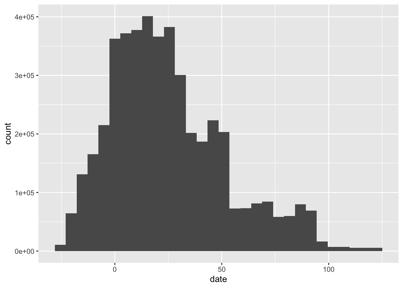
What does this tell you? Add one or more notes:

The distribution shows interaction patterns over time, with some peaks and valleys suggesting different activity levels throughout the course

👉 Your Turn ⤵

Third, please conduct one other data exploration step of your choosing. Options include creating simple graphs or calculating descriptive, summary statistics.

library(skimr)
skim(interactions_filtered)

Data summary
Name	interactions_filtered
Number of rows	4589618
Number of columns	10
_______________________
Column type frequency:
character	3
numeric	7
________________________
Group variables	None

Variable type: character

skim_variable	complete_rate	min	max	n_unique
code_module	1	3	3	7
code_presentation	1	5	5	4
activity_type	1	3	14	19

Variable type: numeric

skim_variable	n_missing	complete_rate	mean	sd	p0	p25	p50	p75	p100	hist
id_student	0	1.00	728767.50	577792.66	6516	508388	586625	644848	2698588	▅▇▁▁▁
id_site	0	1.00	730838.12	129122.13	526721	661804	729683	832712	937844	▇▂▇▅▇
date	0	1.00	25.04	26.99	-25	5	20	41	123	▅▇▃▂▁
sum_click	0	1.00	3.60	8.34	1	1	2	4	6977	▇▁▁▁▁
week_from	3938349	0.14	4.80	4.44	0	2	3	7	29	▇▃▁▁▁
week_to	3938349	0.14	4.84	4.42	0	2	3	7	29	▇▃▁▁▁
quantile_cutoff_date	0	1.00	70.66	25.72	32	51	87	94	124	▅▆▂▇▁

We’re ready to proceed to engineering some features with the interactions data. For the present time, we’ll focus on the sum_click variable, which tells us how many times students clicked on a resource for a given date.

How can we create a feature with sum_click? Think back to our discussion in the presentation; we have many options for working with such time series data. Perhaps the most simple is to count the clicks. Please summarize the number of clicks for each student (specific to a single course). This means you will need to group your data by id_student, code_module, and code_presentation, and then create a summary variable. Assign the resulting output the name interactions_summarized. You may find the documentation for summarize() to be helpful. That is available here. This chapter is also likely helpful (note that summarise() and summarize() are different spellings for the same function).

👉 Your Turn ⤵

interactions_summarized <- interactions_filtered %>% 
    group_by(id_student, code_module, code_presentation) %>% 
    summarize(sum_clicks = sum(sum_click))

`summarise()` has grouped output by 'id_student', 'code_module'. You can
override using the `.groups` argument.

👉 Your Turn ⤵

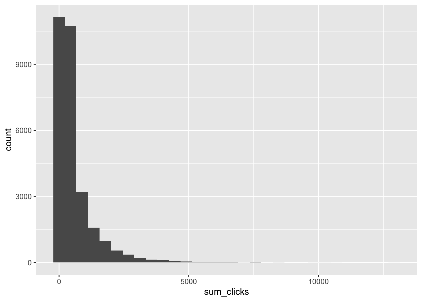
How many times did students click? Let’s create a histogram to see. Please use {ggplot} and geom_histogram() to visualize the distribution of the sum_clicks variable you just created. Turn to the documentation if you need a pointer!

interactions_summarized %>% 
    ggplot(aes(x = sum_clicks)) +
    geom_histogram()

`stat_bin()` using `bins = 30`. Pick better value with `binwidth`.

This is a good start - we’ve created our first feature based upon the log data, sum_clicks! What are some other features we can add? An affordance of using the summarize() function in R is we can create multiple summary statistics at once. Let’s also calculate the standard deviation of the number of clicks as well as the mean. Please copy the code you wrote above into the code chunk below and then add these two additional summary statistics.

👉 Your Turn ⤵

interactions_summarized <- interactions_filtered %>% 
    group_by(id_student, code_module, code_presentation) %>% 
    summarize(sum_clicks = sum(sum_click),
              sd_clicks = sd(sum_click), 
              mean_clicks = mean(sum_click))

`summarise()` has grouped output by 'id_student', 'code_module'. You can
override using the `.groups` argument.

We’ll take one last step here – creating individual slopes of students’ clicks over time. This code is a bit more involved, and so is annotated for you below; feel free to modify and re-use this.

First, we use a custom function that can deal with cases where the fitting of the slopes fails (e.g., for students with only a single data point, or some other unanticipated issue with the model estimation).

# Define a function to fit the model and handle warnings
fit_model <- function(data) {
    tryCatch(
        { 
            # Fit a linear model with sum_click as the response and date as the predictor
            model <- lm(sum_click ~ date, data = data)
            # Tidy the model output (convert to a tidy data frame)
            tidy(model) 
        },
        # Handle errors: return a tibble with NA values
        error = function(e) { tibble(term = NA, estimate = NA, std.error = NA, statistic = NA, p.value = NA) },
        # Handle warnings: return a tibble with NA values
        warning = function(w) { tibble(term = NA, estimate = NA, std.error = NA, statistic = NA, p.value = NA) }
    )
}

Note: this next step may take up to a minute or so! Please feel free to relax!

# Fit the models for each group
interactions_slopes <- interactions_filtered %>%
    group_by(id_student, code_module, code_presentation) %>% # Group by student and course
    nest() %>% # Nest the data frame, creating a list of data frames for each group
    mutate(model = map(data, fit_model)) %>% # Apply the fit_model function to each nested data frame
    unnest(model) # Unnest the model output, returning to a regular data frame

We’ll do a bit of data wrangling.

# Process the output
interactions_slopes <- interactions_slopes %>%
    ungroup() %>% # Remove grouping
    select(code_module, code_presentation, id_student, term, estimate) %>% # Select relevant columns
    filter(!is.na(term)) %>% # Filter out rows where term is NA
    spread(term, estimate) %>% # Spread the terms into separate columns
    mutate_if(is.numeric, round, 4) # Round numeric columns to 4 decimal places

Please rename the resulting intercept and date, changing themintercept and slope, respectively. Note, selecting a variable with a parenthesis in it can be tricky! Think of other ways you could do this, if you wish (hint: think of what a function in janitor can do!).

👉 Your Turn ⤵

interactions_slopes <- interactions_slopes %>% 
    rename(intercept = `(Intercept)`,
           slope = date)

After running this code, we will have intercepts, linear slopes, and quadratic terms for each students’ clickstream pattern over the semester.

Let’s join together several files. First, let’s join all our features into a single file. Please use left_join() to join interactions_summarized and interactions_slopes, assigning the resulting output the name interactions_summarized_and_slopes.

👉 Your Turn ⤵

interactions_summarized_and_slopes <- left_join(interactions_slopes, interactions_summarized)

Joining with `by = join_by(code_module, code_presentation, id_student)`

Just one last step! Let’s join together all of the data we’ll use for our modeling: students_and_assessments and interactions_summarized_and_slopes. Use left_join() once more, assigning the resulting output the name students_assessments_and_interactions. Lots of joining! Sometimes, the hardest part of complex analyses lies in the preparation (and joining) of the data.

👉 Your Turn ⤵

students_assessments_and_interactions <- left_join(students_and_assessments, 
                                                   interactions_summarized_and_slopes)

Joining with `by = join_by(code_module, code_presentation, id_student)`

One more small step. Let’s ensure that our outcome variable – pass – is a factor. It was, but when saving to and reading from a CSV, it lots its factor characteristics, becoming instead a character string. It is necessary for the outcome of a classification model (like the one we are using) to be a factor. Please use mutate() to do just that.

👉 Your Turn ⤵

students_assessments_and_interactions <- students_assessments_and_interactions %>% 
    mutate(pass = as.factor(pass))

students_assessments_and_interactions %>% 
    skimr::skim()

Data summary
Name	Piped data
Number of rows	32593
Number of columns	22
_______________________
Column type frequency:
character	8
factor	1
numeric	13
________________________
Group variables	None

Variable type: character

skim_variable	complete_rate	min	max	n_unique
code_module	1	3	3	7
code_presentation	1	5	5	4
gender	1	1	1	2
region	1	5	20	13
highest_education	1	15	27	5
age_band	1	4	5	3
disability	1	1	1	2
final_result	1	4	11	4

Variable type: factor

skim_variable	n_missing	complete_rate	ordered	n_unique	top_counts
pass	0	1	FALSE	2	0: 20232, 1: 12361

Variable type: numeric

skim_variable	n_missing	complete_rate	mean	sd	p0	p25	p50	p75	p100	hist
id_student	0	1.00	706687.67	549167.31	3733.00	508573.00	590310.00	644453.00	2716795.00	▅▇▁▁▁
imd_band	4627	0.86	5.62	2.73	1.00	4.00	6.00	8.00	10.00	▃▇▇▆▆
num_of_prev_attempts	0	1.00	0.16	0.48	0.00	0.00	0.00	0.00	6.00	▇▁▁▁▁
studied_credits	0	1.00	79.76	41.07	30.00	60.00	60.00	120.00	655.00	▇▁▁▁▁
module_presentation_length	0	1.00	256.01	13.18	234.00	241.00	262.00	268.00	269.00	▇▁▁▅▇
date_registration	45	1.00	-69.41	49.26	-322.00	-100.00	-57.00	-29.00	167.00	▁▂▇▃▁
date_unregistration	22521	0.31	49.76	82.46	-365.00	-2.00	27.00	109.00	444.00	▁▁▇▂▁
mean_weighted_score	7958	0.76	544.70	381.39	0.00	160.00	610.00	875.00	1512.00	▇▃▇▅▁
intercept	3621	0.89	3.08	4.73	-585.59	2.17	2.85	3.75	130.83	▁▁▁▁▇
slope	4409	0.86	0.00	0.21	-12.17	-0.01	0.00	0.02	20.12	▁▇▁▁▁
sum_clicks	3621	0.89	570.23	761.14	1.00	138.00	316.00	667.00	12920.00	▇▁▁▁▁
sd_clicks	3878	0.88	5.01	5.46	0.00	2.43	3.86	6.55	554.90	▇▁▁▁▁
mean_clicks	3621	0.89	3.20	1.28	1.00	2.35	2.97	3.82	46.24	▇▁▁▁▁

We’re now ready to model!

4. MODEL

Step 1. Split data

We’ll follow the same steps we followed in modules #2 and #3, here. One difference - we’ll use students_assessments_and_interactions instead of the data frame we used in those modules. Please port over the code you used in those modules here, changing the name of the data frame to the one we are now using.

We discuss this first step minimally as we have now carried out a step very similar to this in LL1 and LL2; return to the case study for those (especially LL1) for more on data splitting.

👉 Your Turn ⤵

set.seed(2025)

train_test_split <- initial_split(students_assessments_and_interactions, prop = .33, strata = "pass")
data_train <- training(train_test_split)

There is a key difference that is next. In this step. we’ll further process data_train, creating different subsets of the data, or folds of the data, that we can use to fit our model multiple times.

vfcv <- vfold_cv(data_train) # this differentiates this from what we did before
# before, we simple used data_train to fit our model
vfcv

#  10-fold cross-validation 
# A tibble: 10 × 2
   splits              id    
   <list>              <chr> 
 1 <split [9679/1076]> Fold01
 2 <split [9679/1076]> Fold02
 3 <split [9679/1076]> Fold03
 4 <split [9679/1076]> Fold04
 5 <split [9679/1076]> Fold05
 6 <split [9680/1075]> Fold06
 7 <split [9680/1075]> Fold07
 8 <split [9680/1075]> Fold08
 9 <split [9680/1075]> Fold09
10 <split [9680/1075]> Fold10

How does this work? data_train is sampled as many time as we set.

Above, we split the data into 10 different folds. Change the number of folds from 10 to 5 by changing the value of v; 10 is simply the default—not always the best one! For help, run ?vfold_cv to get a hint.

kfcv <- vfold_cv(data_train, v = 5) # Changed from 10 to 5
kfcv

#  5-fold cross-validation 
# A tibble: 5 × 2
  splits              id   
  <list>              <chr>
1 <split [8604/2151]> Fold1
2 <split [8604/2151]> Fold2
3 <split [8604/2151]> Fold3
4 <split [8604/2151]> Fold4
5 <split [8604/2151]> Fold5

Step 2: Engineer features and write down the recipe

Here, we’ll carry out several feature engineering steps.

Read about possible steps and see more about how the following five feature engineering steps below work. Like in the previous learning labs, this is the step in which we set the recipe.

step_normalize(): normalizes numeric data to have a standard deviation of one and a mean of zero
step_dummy(): convert nominal data (e.g. character or factors) into one or more numeric binary model terms for the levels of the original data.
step_impute_knn(): impute missing values using the nearest neighbors method

We will use all three of these. Please note that there are two ways to use each of these. One of them is by specifying the specific variable you want to use for the feature engineering step. For example, below, we would normalize a hypothetical variable, one called minutes_of_videos_watched (note, this code isn’t meant to run!):

step_normalize(minutes_of_videos_watched)

Another way is to specify for which types of variables the feature engineering step applies. You can see all of the available types here. For example, the code below would normalize all numeric variables:

step_normalize(all_numeric_predictors())

👉 Your Turn ⤵

Let’s turn to our recipe. Please add to the code below to add the new variables—features—we created. We’ve started you off with ___ code below (where you can add the new variables – be sure to add all of them!).

my_rec <- recipe(pass ~ disability +
                   date_registration + 
                   gender +
                   code_module +
                   mean_weighted_score +
                   sum_clicks + sd_clicks + mean_clicks + # new
                   intercept + slope, # new
                 data = data_train)

👉 Your Turn ⤵

Then, please add to the following code by completing three steps, building on the code that is started below:

Please normalize all numeric predictors.
Please dummy code the following three variables: disability, gender, and code_module.
Please impute missing values using the nearest neighbors method for the mean_weighted_score, sum_clicks, sd_clicks, mean_clicks, intercept, slope, and date_registration variables.

my_rec <- my_rec %>% 
    step_dummy(disability) %>% 
    step_dummy(gender) %>%  
    step_dummy(code_module) %>% 
    step_impute_knn(mean_weighted_score) %>% 
    step_impute_knn(sum_clicks) %>% 
    step_impute_knn(sd_clicks) %>% 
    step_impute_knn(mean_clicks) %>% 
    step_impute_knn(intercept) %>% 
    step_impute_knn(slope) %>% 
    step_impute_knn(date_registration) %>% 
    step_normalize(all_numeric_predictors())

Step 3: Specify the model and workflow

Next, we specify the model and workflow, using the same engine but a different engine and mode, here, regression for a continuous outcome. Specifically, we are:

using the boost_tree() function to set the model as a boosted tree
using set_engine("xgboost", importance = "gain") to set the engine as that provided for boosted trees through the {xgboost} package; we also add the importance = "gain" line to be able to interpret a variable importance metric specific to boosted tree models
finally, using set_mode("classification")) as we are again predicting categories

# specify model
my_mod <-
  boost_tree(learn_rate = 0.05, trees = 1000, tree_depth = 4) %>%  # boosted tree
  set_engine("xgboost", importance = "gain") %>% # xgboost engine and a variable importance metric
  set_mode("classification")

# specify workflow
my_wf <-
  workflow() %>% # create a workflow
  add_model(my_mod) %>% # add the model we wrote above
  add_recipe(my_rec) # add our recipe we wrote above

Why those defaults? trees: many small steps (1000) learn_rate: 0.05 (smaller → less variance needs more trees) tree_depth: shallow (4) to avoid over‑fitting

Step 4: Fit model

Note that here we use the kfcv data and a different function - fit_resamples(), instead of fit(). This function is required when we have multiple folds of our sample, as we created using the vfcv function above. See more about this function here.

class_metrics <- metric_set(accuracy, sensitivity, specificity, ppv, npv, kap) # specify the same metrics as earlier
fitted_model_resamples <- fit_resamples(my_wf, 
                                        resamples = kfcv, # Changed from vfcv to kfcv
                                        metrics = class_metrics)

Note that you have fit as many models as the value for v that you specified earlier. So, this may take some time. Take a walk, grab a snack, or make a cup of tea!

Then, we can use the same collect_metrics() function we have used to inspect the predictive strength of the model. Please do that for fitted_model_resamples.

👉 Your Turn ⤵

collect_metrics(fitted_model_resamples)

# A tibble: 6 × 6
  .metric     .estimator  mean     n std_err .config             
  <chr>       <chr>      <dbl> <int>   <dbl> <chr>               
1 accuracy    binary     0.658     5 0.00247 Preprocessor1_Model1
2 kap         binary     0.248     5 0.00565 Preprocessor1_Model1
3 npv         binary     0.560     5 0.00239 Preprocessor1_Model1
4 ppv         binary     0.702     5 0.00348 Preprocessor1_Model1
5 sensitivity binary     0.780     5 0.00199 Preprocessor1_Model1
6 specificity binary     0.459     5 0.00699 Preprocessor1_Model1

We noted earlier that we may introduce bias when we evaluate different models against the same training data. The benefit of using the multiple folds - and fitting multiple models - is we can make changes to our features or model. Thus, if we decide to add a new feature, we can run the above steps, without concern about biasing our interpretation of how accurate our model is.

That is, we can be unconcerned about inadvertently introducing bias until we reach the last step - fitting our last model. We can do that using the familiar fit() function, followed by last_fit. It is important to not make further changes after this point.

final_fit <- last_fit(my_wf, train_test_split, metrics = class_metrics)

Step 5: Interpret accuracy

Finally, collect the metrics for our final fit. These are the values that you should report as final.

final_fit %>% 
  collect_metrics()

# A tibble: 6 × 4
  .metric     .estimator .estimate .config             
  <chr>       <chr>          <dbl> <chr>               
1 accuracy    binary         0.661 Preprocessor1_Model1
2 sensitivity binary         0.781 Preprocessor1_Model1
3 specificity binary         0.466 Preprocessor1_Model1
4 ppv         binary         0.705 Preprocessor1_Model1
5 npv         binary         0.565 Preprocessor1_Model1
6 kap         binary         0.255 Preprocessor1_Model1

We can see that final_fit is for a single fit: a boosted tree model with the best performing tuning parameters trained with the entire training set of data to predict the values in our (otherwise not used/“spent”) testing set of data.

👉 Your Turn ⤵

collect_predictions(final_fit) %>% 
    conf_mat(.pred_class, pass)

          Truth
Prediction     0     1
         0 10582  2974
         1  4423  3859

5. COMMUNICATE

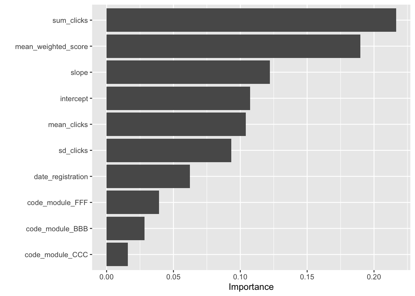
Another benefit of a boosted tree model is we can interpret variable importance metrics. Do that here with the following code.

final_fit %>% 
  pluck(".workflow", 1) %>%   
  extract_fit_parsnip() %>% 
  vip(num_features = 10)

Please add two or more notes on what you notice about which variables (features) are important, focused on what you would say to someone in your audience about what the important variables in your model were.

The mean weighted score remains the most important predictor, similar to the random forest model
The interaction features (sum_clicks, mean_clicks, etc.) show varying levels of importance, indicating that student engagement patterns do contribute to predicting success

🧶 Knit & Check ✅

Congratulations - you’ve completed this case study! Consider moving on to the badge activity next.