Predicting Institutional Graduation Rates Using Testing and Training Data

Case Study

1. PREPARE

We’ll focus on the core parts of doing a machine learning analysis in R, this time bringing into the picture the key concept of training and testing data, which we deliberately omitted from the last case study. We’ll use the {tidymodels} set of R packages (add-ons) to do so, like in the first module. However, to help anchor our analysis and provide us with some direction, we’ll focus on the following research question as we explore this new approach:

How well can we predict which institutions have higher graduation rates?

This builds directly on the work from Module 1, where we started investigating this question. In this module, we’ll properly implement a training and testing workflow to evaluate our predictions more rigorously. We’ll also investigate our data set further to ensure that we understand what goes into the model!

Reading: Statistical modeling: The two cultures

Breiman, L. (2001). Statistical modeling: The two cultures (with comments and a rejoinder by the author). Statistical Science, 16(3), 199-231. https://projecteuclid.org/journals/statistical-science/volume-16/issue-3/Statistical-Modeling--The-Two-Cultures-with-comments-and-a/10.1214/ss/1009213726.pdf

👉 Your Turn ⤵

You’ll be asked to reflect more deeply on this article later on (in the badge activity); but for now, open up the article and take a quick scan of the article and note below an observation or question you have about the article.

• YOUR RESPONSE HERE

Reading: Predicting students’ final grades

Estrellado, R. A., Freer, E. A., Mostipak, J., Rosenberg, J. M., & Velásquez, I. C. (2020). Data science in education using R. Routledge (c14), Predicting students’ final grades using machine learning methods with online course data. http://www.datascienceineducation.com/

Please review this chapter, focusing on the overall goals of the analysis and how the analysis was presented (focusing on predictions, rather than the ways we may typically interpret a statistical model–like measures of statistical significance).

1b. Load Packages

Like in the last module, please load the tidyverse package. Also, please load the tidymodels and janitor packages in the code chunk below. Also, add another package we’ll use, skimr. Install it if you need.

library(tidyverse)

── Attaching core tidyverse packages ──────────────────────── tidyverse 2.0.0 ──
✔ dplyr     1.1.4     ✔ readr     2.1.5
✔ forcats   1.0.0     ✔ stringr   1.5.1
✔ ggplot2   3.5.2     ✔ tibble    3.3.0
✔ lubridate 1.9.3     ✔ tidyr     1.3.1
✔ purrr     1.0.4     
── Conflicts ────────────────────────────────────────── tidyverse_conflicts() ──
✖ dplyr::filter() masks stats::filter()
✖ dplyr::lag()    masks stats::lag()
ℹ Use the conflicted package (<http://conflicted.r-lib.org/>) to force all conflicts to become errors

library(tidymodels)

── Attaching packages ────────────────────────────────────── tidymodels 1.2.0 ──
✔ broom        1.0.7      ✔ rsample      1.2.1 
✔ dials        1.2.1      ✔ tune         1.2.1 
✔ infer        1.0.7      ✔ workflows    1.1.4 
✔ modeldata    1.4.0      ✔ workflowsets 1.1.0 
✔ parsnip      1.2.1      ✔ yardstick    1.3.1 
✔ recipes      1.0.10     
── Conflicts ───────────────────────────────────────── tidymodels_conflicts() ──
✖ scales::discard() masks purrr::discard()
✖ dplyr::filter()   masks stats::filter()
✖ recipes::fixed()  masks stringr::fixed()
✖ dplyr::lag()      masks stats::lag()
✖ yardstick::spec() masks readr::spec()
✖ recipes::step()   masks stats::step()
• Use tidymodels_prefer() to resolve common conflicts.

library(janitor)

Attaching package: 'janitor'

The following objects are masked from 'package:stats':

    chisq.test, fisher.test

library(skimr)

2. WRANGLE

In general, data wrangling involves some combination of cleaning, reshaping, transforming, and merging data (Wickham & Grolemund, 2017). The importance of data wrangling is difficult to overstate, as it involves the initial steps of going from raw data to a dataset that can be explored and modeled (Krumm et al, 2018). In Part 2, we focus on the following wrangling processes to:

1. Importing and Inspecting Data. In this section, we will “read” in our CSV data file and take a quick look at what our file contains.

2. Transform Variables. We use the mutate() function to create a dichotomous variable for whether or not the institution has a “good” graduation rate, building on what we did in Module 1.

2a. Import and Inspect Data

For this module, we’ll be working with the same IPEDS (Integrated Postsecondary Education Data System) dataset we used in Module 1. Let’s read it in:

ipeds <- read_csv("data/ipeds-all-title-9-2022-data.csv")

Rows: 5988 Columns: 24
── Column specification ────────────────────────────────────────────────────────
Delimiter: ","
chr  (9): institution name, HD2022.Postsecondary and Title IV institution in...
dbl (15): unitid, year, DRVADM2022.Percent admitted - total, DRVIC2022.Tuiti...

ℹ Use `spec()` to retrieve the full column specification for this data.
ℹ Specify the column types or set `show_col_types = FALSE` to quiet this message.

We’ll use the same data cleaning steps from Module 1:

ipeds <- clean_names(ipeds)

ipeds <- ipeds %>% 
    select(name = institution_name, 
           title_iv = hd2022_postsecondary_and_title_iv_institution_indicator, # is the university a title IV university?
           carnegie_class = hd2022_carnegie_classification_2021_basic, # which carnegie classification
           state = hd2022_state_abbreviation, # state
           total_enroll = drvef2022_total_enrollment, # total enrollment
           pct_admitted = drvadm2022_percent_admitted_total, # percentage of applicants admitted
           n_bach = drvc2022_bachelors_degree, # number of students receiving a bachelor's degree
           n_mast = drvc2022_masters_degree, # number receiving a master's
           n_doc = drvc2022_doctors_degree_research_scholarship, # number receive a doctoral degree
           tuition_fees = drvic2022_tuition_and_fees_2021_22, # total cost of tuition and fees
           grad_rate = drvgr2022_graduation_rate_total_cohort, # graduation rate
           percent_fin_aid = sfa2122_percent_of_full_time_first_time_undergraduates_awarded_any_financial_aid, # percent of students receive financial aid
           avg_salary = drvhr2022_average_salary_equated_to_9_months_of_full_time_instructional_staff_all_ranks) # average salary of instructional staff

👉 Your Turn ⤵

Just as we did in Module 1, let’s filter the data to include only Title IV postsecondary institutions.

ipeds <- ipeds %>% 
    filter(title_iv == "Title IV postsecondary institution")

👉 Your Turn ⤵

Now, filter the data again to only include institutions with a carnegie classification. Specifically, exclude those institutions with a value for the carnegie_class variable that is “Not applicable, not in Carnegie universe (not accredited or nondegree-granting)”. As a hint: whereas the logical operator == is used to include only matching conditions, the logical operator != excludes matching conditions.

ipeds <- ipeds %>% 
    filter(carnegie_class != "Not applicable, not in Carnegie universe (not accredited or nondegree-granting)")

👉 Your Turn ⤵

Let’s inspect our data - using glimpse() or another means of your choosing below.

glimpse(ipeds)

Rows: 3,818
Columns: 13
$ name            <chr> "Alabama A & M University", "University of Alabama at …
$ title_iv        <chr> "Title IV postsecondary institution", "Title IV postse…
$ carnegie_class  <chr> "Master's Colleges & Universities: Larger Programs", "…
$ state           <chr> "Alabama", "Alabama", "Alabama", "Alabama", "Alabama",…
$ total_enroll    <dbl> 6007, 21639, 647, 9237, 3828, 38644, 1777, 2894, 5109,…
$ pct_admitted    <dbl> 68, 87, NA, 78, 97, 80, NA, NA, 92, 44, 57, NA, NA, NA…
$ n_bach          <dbl> 511, 2785, 54, 1624, 480, 6740, NA, 738, 672, 5653, 26…
$ n_mast          <dbl> 249, 2512, 96, 570, 119, 2180, NA, 80, 300, 1415, 0, N…
$ n_doc           <dbl> 9, 166, 20, 41, 2, 215, NA, 0, 0, 284, 0, NA, 0, NA, N…
$ tuition_fees    <dbl> 10024, 8568, NA, 11488, 11068, 11620, 4930, NA, 8860, …
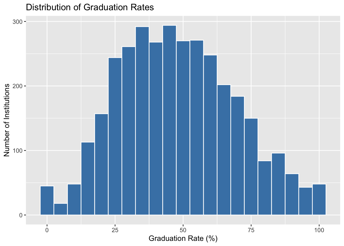
$ grad_rate       <dbl> 27, 64, 50, 63, 28, 73, 22, NA, 36, 81, 65, 26, 9, 29,…
$ percent_fin_aid <dbl> 87, 96, NA, 96, 97, 87, 87, NA, 99, 79, 100, 96, 92, 8…
$ avg_salary      <dbl> 77824, 106434, 36637, 92561, 72635, 97394, 63494, 8140…

Write down a few observations after inspecting the data:

• YOUR RESPONSE HERE
• YOUR RESPONSE HERE
• YOUR RESPONSE HERE

2b. Transform Variables

We’ll now transform our graduation rate variable into a binary outcome for our classification task, just as we did in Module 1.

👉 Your Turn ⤵

Create a binary variable called good_grad_rate that indicates whether an institution has a graduation rate above a certain threshold. Choose a threshold that seems reasonable to you.

ipeds <- ipeds %>% 
    mutate(good_grad_rate = if_else(grad_rate > 62, 1, 0),
           good_grad_rate = as.factor(good_grad_rate))

Here, add a reason or two for how and why you picked the threshold you did:

• YOUR RESPONSE HERE
• YOUR RESPONSE HERE

3. EXPLORE

As noted by Krumm et al. (2018), exploratory data analysis often involves some combination of data visualization and feature engineering. In Part 3, we will create a quick visualization to help us spot any potential issues with our data and engineer new predictive variables or “features” that we will use in our predictive models.

3a. Examine Variables

Let’s take a closer look at our institutional data. In the chunk below, count the number of institutions with good and poor graduation rates.

ipeds %>% 
    count(good_grad_rate)

# A tibble: 3 × 2
  good_grad_rate     n
  <fct>          <int>
1 0               2529
2 1                871
3 <NA>             418

What does this tell us?

We can use the tabyl function to explore a bit further:

ipeds %>% 
    tabyl(good_grad_rate)

 good_grad_rate    n   percent valid_percent
              0 2529 0.6623887     0.7438235
              1  871 0.2281299     0.2561765
           <NA>  418 0.1094814            NA

We can see how many institutions have good and not-so-good graduations rates – and what percentage of the data is missing.

Next, let’s visualize the distribution of graduation rates to better understand our data:

ipeds %>% 
    ggplot(aes(x = grad_rate)) +
    geom_histogram(binwidth = 5, fill = "steelblue", color = "white") +
    labs(title = "Distribution of Graduation Rates",
         x = "Graduation Rate (%)",
         y = "Number of Institutions")

Warning: Removed 418 rows containing non-finite outside the scale range
(`stat_bin()`).

👉 Your Turn ⤵

Create another visualization that explores the relationship between two variables in our dataset. For example, you might want to look at the relationship between tuition fees and graduation rates, or enrollment and graduation rates.

# Add your visualization code here

One last, critical step is understanding missingness in our data. The skim() function from the {skimr} package is fantastic for this — it tells us the number and percentage of missing values for each variable in our data set.

skim(ipeds)

Data summary

Name	ipeds
Number of rows	3818
Number of columns	14
_______________________
Column type frequency:
character	4
factor	1
numeric	9
________________________
Group variables	None

Variable type: character

skim_variable	n_missing	complete_rate	min	max	empty	n_unique	whitespace
name	0	1	6	91	0	3775	0
title_iv	0	1	34	34	0	1	0
carnegie_class	0	1	15	88	0	33	0
state	0	1	4	30	0	59	0

Variable type: factor

skim_variable	n_missing	complete_rate	ordered	n_unique	top_counts
good_grad_rate	418	0.89	FALSE	2	0: 2529, 1: 871

Variable type: numeric

skim_variable	n_missing	complete_rate	mean	sd	p0	p25	p50	p75	p100	hist
total_enroll	0	1.00	4884.67	9327.97	1	532	1796.5	5058.00	164091	▇▁▁▁▁
pct_admitted	2040	0.47	71.86	22.51	0	60	77.0	89.00	100	▁▁▃▆▇
n_bach	1192	0.69	771.19	1672.82	0	25	209.0	649.75	24230	▇▁▁▁▁
n_mast	1195	0.69	336.29	922.00	0	0	47.0	273.50	19615	▇▁▁▁▁
n_doc	1195	0.69	30.38	112.18	0	0	0.0	4.00	1595	▇▁▁▁▁
tuition_fees	599	0.84	16801.79	15347.31	480	5039	10830.0	25045.00	66064	▇▂▂▁▁
grad_rate	418	0.89	48.11	21.62	0	32	47.0	63.00	100	▂▇▇▅▂
percent_fin_aid	405	0.89	89.88	15.56	0	86	97.0	100.00	100	▁▁▁▁▇
avg_salary	113	0.97	67775.88	24347.24	1	52170	64822.0	80244.00	215232	▂▇▂▁▁

From this, we can see that several variables have considerable missingness. For example, the pct_admitted variable has more than half of its values missing! There are ways to deal with this (real-life datasets, including the IPEDS data, are rife with missing values for a whole host of reasons). We will address those (e.g., imputation) later.

For this analysis, though, we’ll focus on the variables that have relatively few missing values - tuition_fees, percent_fin_aid, avg_salary, and our dependent variable, good_grad_rate. This will be a simple model — simpler in terms of the features than the model in the first analysis, but with the knowledge that we are using variables that are more complete.

3b. Feature Engineering

As defined by Krumm, Means, and Bienkowski (2018) in Learning Analytics Goes to School:

Feature engineering is the process of creating new variables within a dataset, which goes above and beyond the work of recoding and rescaling variables.

The authors note that feature engineering draws on substantive knowledge from theory or practice, experience with a particular data system, and general experience in data-intensive research. Moreover, these features can be used not only in machine learning models, but also in visualizations and tables comprising descriptive statistics.

Though not as often discussed as other steps, feature engineering is an important step. You can read more about feature engineering here.

For this module, we’ll create a new feature that might help predict graduation rates. Let’s create a derived variable representing the ratio of tuition and fees to average salary, which could indicate the institution’s value proposition.

ipeds <- ipeds %>% 
    mutate(tuition_to_salary_ratio = tuition_fees / avg_salary)

Let’s examine this new feature:

ipeds %>% 
    ggplot(aes(x = tuition_to_salary_ratio, fill = good_grad_rate)) +
    geom_density()

Warning: Removed 656 rows containing non-finite outside the scale range
(`stat_density()`).

Something is very not right. It seems like there may be some number that is way off – and that’s skewing the plot in a weird way.

What’s going on? In this case, it can be helpful to get eyes on the data to see if anything funny seems to be going on. Let’s take a look at the relevant variables:

select(ipeds, name, tuition_fees, avg_salary, tuition_to_salary_ratio) %>% 
    arrange((desc(tuition_to_salary_ratio)))

# A tibble: 3,818 × 4
   name                           tuition_fees avg_salary tuition_to_salary_ra…¹
   <chr>                                 <dbl>      <dbl>                  <dbl>
 1 Beckfield College-Florence            13295          1               13295   
 2 Young Americans College of th…        14030       5854                   2.40
 3 Los Angeles Academy of Figura…        31618      17175                   1.84
 4 Aviator College of Aeronautic…        31211      19335                   1.61
 5 Williamson Christian College          13730       9000                   1.53
 6 Ecclesia College                      15950      11762                   1.36
 7 Millennia Atlantic University         11992       9225                   1.30
 8 Beverly Hills Design Institute        23220      18750                   1.24
 9 Ohio Christian University             22506      19010                   1.18
10 Longy School of Music of Bard…        48800      45370                   1.08
# ℹ 3,808 more rows
# ℹ abbreviated name: ¹​tuition_to_salary_ratio

Do you spot the problem? Add a note below about what it might be:

• YOUR RESPONSE HERE

As you likely noticed, it looks like one institution - Beckfield College-Florence - has an average salary of $1 for their graduates. As a result, the ratio of tuition and fees relative to salary is huge – far larger than for any other institutions! What to do here? This seems almost certain to be an error in data reporting or recording. We can safely filter out this one row with some simple logic.

ipeds <- ipeds %>% 
    filter(avg_salary > 1)

Let’s try to create that plot again:

ipeds %>% 
    ggplot(aes(x = tuition_to_salary_ratio, fill = good_grad_rate)) +
    geom_density()

Warning: Removed 543 rows containing non-finite outside the scale range
(`stat_density()`).

That’s better! Add a note on what this graph might mean below:

• YOUR RESPONSE HERE

We’re now ready to proceed to the five machine learning (modeling) steps!

4. MODEL

In this step, we will dive into the SML modeling process in much more depth than in the last module.

1. Split Data into a training and test set that will be used to develop a predictive model;

2. Create a “Recipe” for our predictive model and learn how to deal with nominal data that we would like to use as predictors;

3. Specify the model and workflow by selecting the functional form of the model that we want and using a model workflow to pair our model and recipe together;

4. Fit Models to our training set using logistic regression;

5. Interpret Accuracy of our model to see how well our model can “predict” our outcome of interest.

Step 1. Split data

We didn’t split the data we used in the first module. Instead, we used data to train our model, and then we used the same data set to evaluate how good our model performed, i.e., to test our model. This raises an issue: using the same data to train and test our model can lead to something called overfitting, which is when a model learns the specifics in the training data rather than the underlying pattern.

This is related to the bias-variance trade off introduced in the conceptual overview: by using the same data to train and test our model, we run the risk of developing a model with low bias, but high variance. Any changes in the training data could result in a very different model (with far higher bias), which is not ideal. In other words, we want to develop a model that is generalizable to new data, not just the data we used to train it.

The authors of Data Science in Education Using R (Estrellado et al., 2020) remind us that:

At its core, machine learning is the process of “showing” your statistical model only some of the data at once and training the model to predict accurately on that training dataset (this is the “learning” part of machine learning). Then, the model as developed on the training data is shown new data - data you had all along, but hid from your computer initially - and you see how well the model that you developed on the training data performs on this new testing data. Eventually, you might use the model on entirely new data.

Training and Testing Sets

It is therefore common when beginning a modeling project to separate the data set into two partitions:

• The training set is used to estimate, develop and compare models; feature engineering techniques; tune models, etc.

• The test set is held in reserve until the end of the project, at which point there should only be one or two models under serious consideration. It is used as an unbiased source for measuring final model performance.

There are different ways to create these partitions of the data and there is no uniform guideline for determining how much data should be set aside for testing. The proportion of data can be driven by many factors, including the size of the original pool of samples and the total number of predictors.

After you decide how much to set aside, the most common approach for actually partitioning your data is to use a random sample. For our purposes, we’ll use random sampling to select 20% for the test set and use the remainder for the training set, which are the defaults for the {rsample} package.

Split Data Sets

To split our data, we will be using our first {tidymodels} function - initial_split().

The function initial_split() function from the {rsample} package takes the original data and saves the information on how to make the partitions. The {rsample} package has two aptly named functions for created a training and testing data set called training() and testing(), respectively.

We also specify the strata to ensure there is not misbalance in the dependent variable (good_grad_rate).

Run the following code to split the data:

set.seed(20250712)

train_test_split <- initial_split(ipeds, prop = .80, strata = "good_grad_rate")

data_train <- training(train_test_split)

data_test  <- testing(train_test_split)

Note: Since random sampling uses random numbers, it is important to set the random number seed using the set.seed() function. This ensures that the random numbers can be reproduced at a later time (if needed). We pick the first date on which we may carry out this learning lab as the seed, but any number will work!

👉 Your Turn ⤵

Go ahead and type data_train and data_test into the console (in steps) to check that this data set indeed has 80% of the number of observations as in the larger data. Do that in the chunk below:

data_train

# A tibble: 2,962 × 15
   name    title_iv carnegie_class state total_enroll pct_admitted n_bach n_mast
   <chr>   <chr>    <chr>          <chr>        <dbl>        <dbl>  <dbl>  <dbl>
 1 Amridg… Title I… Master's Coll… Alab…          647           NA     54     96
 2 Alabam… Title I… Doctoral/Prof… Alab…         3828           97    480    119
 3 Centra… Title I… Associate's C… Alab…         1777           NA     NA     NA
 4 Auburn… Title I… Master's Coll… Alab…         5109           92    672    300
 5 Chatta… Title I… Associate's C… Alab…         1641           NA     NA     NA
 6 South … Title I… Baccalaureate… Alab…          361           NA     31     17
 7 Enterp… Title I… Associate's C… Alab…         2010           NA     NA     NA
 8 Coasta… Title I… Associate's C… Alab…         6800           NA     NA     NA
 9 George… Title I… Associate's C… Alab…         3832           NA     NA     NA
10 George… Title I… Associate's C… Alab…         5965           NA     NA     NA
# ℹ 2,952 more rows
# ℹ 7 more variables: n_doc <dbl>, tuition_fees <dbl>, grad_rate <dbl>,
#   percent_fin_aid <dbl>, avg_salary <dbl>, good_grad_rate <fct>,
#   tuition_to_salary_ratio <dbl>

data_test

# A tibble: 742 × 15
   name    title_iv carnegie_class state total_enroll pct_admitted n_bach n_mast
   <chr>   <chr>    <chr>          <chr>        <dbl>        <dbl>  <dbl>  <dbl>
 1 Alabam… Title I… Master's Coll… Alab…         6007           68    511    249
 2 Athens… Title I… Baccalaureate… Alab…         2894           NA    738     80
 3 Auburn… Title I… Doctoral Univ… Alab…        31764           44   5653   1415
 4 Faulkn… Title I… Master's Coll… Alab…         2817           82    448    347
 5 Gadsde… Title I… Associate's C… Alab…         4352           NA     NA     NA
 6 Huntin… Title I… Baccalaureate… Alab…          817           66    204      0
 7 Univer… Title I… Master's Coll… Alab…         1804           84    210     96
 8 Univer… Title I… Master's Coll… Alab…         2586           60    414    126
 9 Snead … Title I… Associate's C… Alab…         2507           NA     NA     NA
10 Alaska… Title I… Special Focus… Alas…          268           NA     NA     NA
# ℹ 732 more rows
# ℹ 7 more variables: n_doc <dbl>, tuition_fees <dbl>, grad_rate <dbl>,
#   percent_fin_aid <dbl>, avg_salary <dbl>, good_grad_rate <fct>,
#   tuition_to_salary_ratio <dbl>

Step 2: Create a “Recipe”

In this section, we introduce another tidymodels package named {recipes}, which is designed to help you prepare your data before training your model. Recipes are built as a series of preprocessing steps, such as:

• converting qualitative predictors to indicator variables (also known as dummy variables),

• transforming data to be on a different scale (e.g., taking the logarithm of a variable),

• transforming whole groups of predictors together,

• extracting key features from raw variables (e.g., getting the day of the week out of a date variable), and so on.

If you are familiar with R’s formula interface, a lot of this might sound familiar and like what a formula already does. Recipes can be used to do many of the same things, but they have a much wider range of possibilities.

We’ll dive more into the above steps in later modules, focusing on the formula for our model at this point. So, for now, we’ll simply add the features we used in the last module, adding the new feature we created above.

Add a formula

To get started, let’s create a recipe for a simple logistic regression model. Before training the model, we can use a recipe.

The recipe()function as we used it here has two arguments:

• A formula. Any variable on the left-hand side of the tilde (~) is considered the model outcome (code, in our present case). On the right-hand side of the tilde are the predictors. Variables may be listed by name, or you can use the dot (.) to indicate all other variables as predictors. This is where we can add functions to automate some of the feature engineering steps (in later modules).

• The data. A recipe is associated with the data set used to create the model. This will typically be the training set, so data = train_data here. Naming a data set doesn’t actually change the data itself; it is only used to catalog the names of the variables and their types, like factors, integers, dates, etc.

👉 Your Turn ⤵

Let’s create a recipe where we predict good_grad_rate (the outcome variable) on the basis of several variables:

• tuition_fees
• avg_salary
• percent_fin_aid
• tuition_to_salary_ratio (the variable we created based on two of the above variables)

my_rec <- recipe(good_grad_rate ~ 
                     tuition_fees +
                     avg_salary +
                     tuition_to_salary_ratio +
                     percent_fin_aid,
                 data = ipeds) 

Step 3: Specify the model and workflow

With tidymodels, we start building a model by specifying the functional form of the model that we want using the {parsnip} package. Since our outcome is binary, the model type we will use is “logistic regression.” We can declare this with logistic_reg() and assign to an object we will later use in our workflow:

Run the following code to finish specifying our model:

# specify model
my_mod <-
    logistic_reg()

That is pretty underwhelming since, on its own, it doesn’t really do much. However, now that the type of model has been specified, a method for fitting or training the model can be stated using the engine.

Start your engine

To set the engine, let’s rewrite the code above and “pipe” in the set_engine("glm") function and set_mode("classification")) to set the “mode” to classification. Note that this could also be changed to regression for a continuous/numeric outcome.

👉 Your Turn ⤵

Below, specify a glm engine, and a classification mode, replacing the placeholder text below.

my_mod <-
    logistic_reg() %>% 
    set_engine("glm") %>% # generalized linear model
    set_mode("classification") # since we are predicting a dichotomous outcome, specify classification; for a number, specify regression

my_mod

Logistic Regression Model Specification (classification)

Computational engine: glm 

The engine value is often a mash-up of different packages that can be used to fit or train the model as well as the estimation method. For example, we will use “glm” a generalized linear model for binary outcomes and default for logistic regression in the {parsnip} package.

Add to workflow

Now we can use the recipe created earlier across several steps as we train and test our model. To simplify this process, we can use a model workflow, which pairs a model and recipe together.

This is a straightforward approach because different recipes are often needed for different models, so when a model and recipe are bundled, it becomes easier to train and test workflows.

We’ll use the{workflows} package from tidymodels to bundle our parsnip model (lr_mod) with our first recipe (lr_recipe_1).

Add your model and recipe (see their names above)!

my_wf <-
    workflow() %>% # create a workflow
    add_model(my_mod) %>% # add the model we wrote above
    add_recipe(my_rec) # add our recipe we wrote above

Step 4: Fit model

Now that we have a single workflow that can be used to prepare the recipe and train the model from the resulting predictors, we can use the fit() function to fit our model to our train_data. And again, we set a random number seed to ensure that if we run this same code again, we will get the same results in terms of the data partition:

Finally, we’ll use the last_fit function, which is the key here: note that it uses the train_test_split data—not just the training data.

Here, then, we fit the data using the training data set and evaluate its accuracy using the testing data set (which is not used to train the model), passing the my_wf object as the first argument, and the split as the second.

final_fit <- last_fit(my_wf, train_test_split)

👉 Your Turn ⤵

Type the output of the above function (the name you assigned the output to) below; this is the final, fitted model—one that can be interpreted further in the next step!

final_fit

# Resampling results
# Manual resampling 
# A tibble: 1 × 6
  splits             id               .metrics .notes   .predictions .workflow 
  <list>             <chr>            <list>   <list>   <list>       <list>    
1 <split [2962/742]> train/test split <tibble> <tibble> <tibble>     <workflow>

You may see a message/warning above or when you examine final_fit; you can safely ignore that.

Step 5: Interpret accuracy

Importantly, we can summarize across all of these codes. One way to do this is straightforward; how many of the codes were the same, as in the following chunk of code:

final_fit %>% 
    collect_predictions() %>% # see test set predictions
    select(.pred_class, good_grad_rate) %>% # just to make the output easier to view 
    mutate(correct = .pred_class == good_grad_rate) # create a new variable, co

# A tibble: 742 × 3
   .pred_class good_grad_rate correct
   <fct>       <fct>          <lgl>  
 1 0           0              TRUE   
 2 <NA>        <NA>           NA     
 3 0           1              FALSE  
 4 0           0              TRUE   
 5 0           0              TRUE   
 6 0           0              TRUE   
 7 0           0              TRUE   
 8 0           0              TRUE   
 9 0           0              TRUE   
10 <NA>        1              NA     
# ℹ 732 more rows

You may notice some of the rows may be missing values. This is because there were some missing values in the imd_band variable, and for this machine learning algorithm (the generalized linear model), missing values result in row-wise deletion.

When these are the same, the model predicted the code correctly; when they aren’t the same, the model was incorrect.

We can also tabulate these using the tabyl function:

final_fit %>% 
    collect_predictions() %>% # see test set predictions
    select(.pred_class, good_grad_rate) %>% # just to make the output easier to view 
    mutate(correct = .pred_class == good_grad_rate) %>%  # create a new variable, co
    tabyl(correct)

 correct   n   percent valid_percent
   FALSE  98 0.1320755     0.1573034
    TRUE 525 0.7075472     0.8426966
      NA 119 0.1603774            NA

👉 Your Turn ⤵

A short-cut to the above is to simply use the collect_metrics() function, taking final_fit as its one argument; we’ll use this short-cut from here forward, having seen how accuracy is calculated. Write that code below.

collect_metrics(final_fit)

# A tibble: 3 × 4
  .metric     .estimator .estimate .config             
  <chr>       <chr>          <dbl> <chr>               
1 accuracy    binary         0.843 Preprocessor1_Model1
2 roc_auc     binary         0.844 Preprocessor1_Model1
3 brier_class binary         0.118 Preprocessor1_Model1

Let’s step back a bit. How well could we do if we include more data? And how useful could such a model be in the real world? We’ll dive into these questions more over the forthcoming modules.

That’s it for now; the core parts of machine learning are used in the above steps you took; what we’ll do after this leaning lab only adds nuance and complexity to what we’ve already done.

5. COMMUNICATE

For your SML Module 2 Badge, you will have an opportunity to create a simple “data product” designed to illustrate insights some insights gained from your model and ideally highlight an “action step” that can be taken to act upon your findings.

Rendered HTML files can be published online through a variety of ways including Posit Cloud, RPubs , GitHub Pages, Quarto Pub, or other methods. The easiest way to quickly publish your file online is to publish directly from RStudio. You can do so by clicking the “Publish” button located in the Viewer Pane after you render your document as illustrated in the screenshot below.

Congratulations - you’ve completed the second supervised machine learning case study!