Components, Cliques, and Key-Actors

SNA Module 3: Code-Along

Overview

Prepare: Review the #COMMONCORE project including questions, data, and key findings.
Wrangle: Revisit basic techniques for manipulating, cleaning, transforming, and merging network data.
Explore: Calculate some key measures for individuals in our network and illustrate key actors through network visualization.
Model: Introduce community detection algorithms for identifying groups.
Communicate: Discuss website as a format for sharing findings.

Prepare

Introduction to #COMMONCORE

Our third SNA learning lab is inspired by the #commoncore Project, which examined the intense debate surrounding the Common Core State Standards education reform as it played out on Twitter.

The central question guiding the #COMMONCORE Project was:

How are social media-enabled social networks changing the discourse in American politics that produces and sustains education policy?

The authors used Twitter’s (now X’s, now sadly defunct) Application Programming Interface (API) based on tweets using specified keywords, keyphrases, or hashtags and then restricted their analysis to the following terms: commoncore, ccss and stopcommoncore.
They also captured Twitter profile names, or user names, as well as the tweets, retweets, and mentions posted.

In Act 1, The Giant Network, the authors identified five major sub-communities, or factions, including: (1) supporters, (2) opponents inside education, and (3) opponents outside of education.
In Act 2, Central Actors, they noted that most of these participants were casual contributors and distinguished between two types of central actors on Twitter: Transmitters and Transceivers.

Wrangle

Import, Inspect, and Tidy Network Data

Inspect Data

Load Libraries
Import Data
Inspect Data
Discuss

Let’s start by creating a new R script and loading the following packages introduced in previous modules:

library(tidyverse)
library(igraph)
library(tidygraph)
library(ggraph)

# You may have to install this package if it is not listed in your packages pane.
# install.packages(tidyverse)

Run the following code to use the read_csv() function from the {readr} package to read the ccss-tweets-fresh.csv file from the data folder and assign to a new data frame named ccss_tweets:

ccss_ties <- read_csv("module-1/data/ccss-edgelist.csv")
ccss_nodes <- read_csv("module-1/data/ccss-nodelist.csv")

Now let’s take a look at the data file we just imported using the View() function or another function of choice you may have learned in the Foundations Labs:

view(ccss_ties)
view(ccss_nodes)

Think about the questions below and be prepared to share your response:

What do you think the rows and columns in each file represent?
What about the values in each cell represent?
What else do you notice about the data?
What questions do you have?

Tidy Data

tbl_graph() function
Inspect Graph
View Sociogram
Output
Discuss

The tbl_graph() function creates a special network data structure called a “tidy graph” that combines our nodes and edges into a single R object. Run the following code in your R script:

Using your R script, type the name of network object we just created and run the code to produce the output on the next tab:

# YOUR TURN
#
#

ggraph(ccss_network, layout = "fr") + 
  geom_edge_link(arrow = arrow(length = unit(1, 'mm')), 
                 end_cap = circle(3, 'mm'),
                 start_cap = circle(3, 'mm'),
                 alpha = .1) +
  geom_node_point(aes(size = local_size())) +
  geom_node_text(aes(label = actors,
                     size = local_size()),
                 repel=TRUE) +
  theme_graph()

Think about the questions below:

What is size of our CSSS twitter network?
Does our network contain any obvious groups?
What insights have gained about out network so far?
What questions do have about have about out network so far?

Explore

Components, Cliques, & Key Actors

Components

Definition
Quick Look
Output
Implementation
Interpret

One of the most basic ways researchers can characterize a network’s substructure is to identify its components.

A component is a connected subgraph in which there is a path between all pairs of nodes.

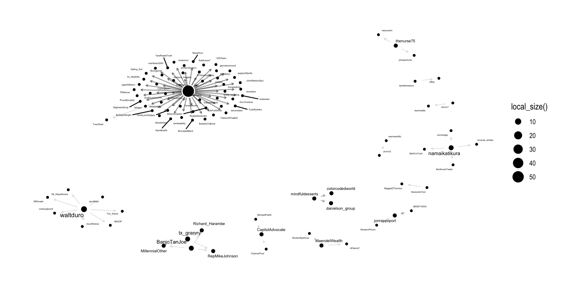
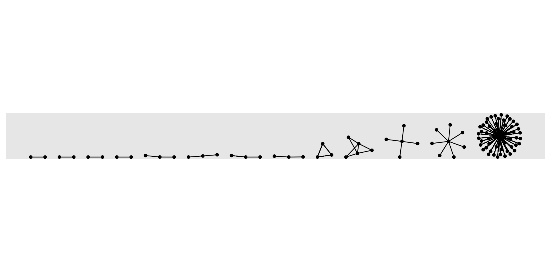
Recall from our output above that our directed “multigraph” had 13 components.

A weak component, as illustrated by the graph generated by the code below, ignores the direction of a tie:

autograph(ccss_network)

Strong components do not. In other words:

Strong components consist of nodes that are connected to one another via both directions along the path that connects them.

The {igraph} package has a simple components() function for identifying the number of components in a network, the size of each component, and which actors belong to each.

components(ccss_network, mode = c("strong"))

How many “strong” components are in our network?

$membership
 [1] 91 92 86 87 90 89 88 84 85 81 83 82 73 80 79 78 77 76 75 74 71 72 70 69 67
[26] 68 62 66 65 64 63 59 61 60 56 57 58  5 55 54 53 52 51 50 49 48 47 46 45 44
[51] 43 42 41 40 39 38 37 36 35 34 33 32 31 30 29 28 27 26 25 24 23 22 21 20 19
[76] 18 17 16 15 14 13 12 11 10  9  8  7  6  3  4  1  2

$csize
 [1] 1 1 1 1 1 1 1 1 1 1 1 1 1 1 1 1 1 1 1 1 1 1 1 1 1 1 1 1 1 1 1 1 1 1 1 1 1 1
[39] 1 1 1 1 1 1 1 1 1 1 1 1 1 1 1 1 1 1 1 1 1 1 1 1 1 1 1 1 1 1 1 1 1 1 1 1 1 1
[77] 1 1 1 1 1 1 1 1 1 1 1 1 1 1 1 1

$no
[1] 92

Cliques

Definition
Clique Number
Implementation
Interpret

Examining cliques is one bottom-up approach that reveals how groups are distributed in the network and which actors belong to which groups.

A clique is a maximally connected subgraph of nodes (> 2) in which all nodes are connected to each other.

Similar to our component analysis, the {igraph} function has a super simple clique_num() function for identifying number of completely connected subgroups in a network:

clique_num(ccss_network)

As you probably saw above, the clique_num() function does not take into account directionality of our ties. It looks like we have 3 clusters of at least 3 actors that all have ties to one another.

The {igraph} function also has a simple cliques() function for identifying members who belong to the same group.

Let’s see if there are any cliques that contain a minimum of 3 nodes?

cliques(ccss_network, min = 3, max = NULL)

[[1]]
+ 3/92 vertices, from a958a0b:
[1] 35 36 37

[[2]]
+ 3/92 vertices, from a958a0b:
[1] 3 4 7

[[3]]
+ 3/92 vertices, from a958a0b:
[1] 3 4 6

[[4]]
+ 3/92 vertices, from a958a0b:
[1] 3 4 5

Key Actors

Degree
Activate Nodes
View Network
Your Turn
Answer

As we learned in our previous lab, a key structural property of networks is the concept of centralization.

One of the most common descriptives reported in network studies and a primary measure of centralization is degree.

Degree is the number of ties to and from an ego. In a directed network, in-degree is the number of ties received, whereas out-degree is the number of ties sent.

The {tidygraph} package has an aptly named function centrality_degree() for calculating degree, in-degree, and out-degree for all actors in a network.

To use it, we’ll need to activate() our nodes and create a new node-level variable using mutate() from the {dplyr} package:

ccss_network <- ccss_network |>
  activate(nodes) |>
  mutate(in_degree = centrality_degree(mode = "in"),
         out_degree = centrality_degree(mode = "out"))

Let’s take a look at our network now.

ccss_network

# A tbl_graph: 92 nodes and 289 edges
#
# A directed multigraph with 13 components
#
# A tibble: 92 × 3
  actors          in_degree out_degree
  <chr>               <dbl>      <dbl>
1 AlexiosAsText           0          1
2 MaggieEThornton         1          0
3 tx_granny               0          4
4 BanjoTanJoe             1          3
5 MillennialOther         2          0
6 Richard_Harambe         2          0
# ℹ 86 more rows
#
# A tibble: 289 × 4
   from    to created_at          text                                          
  <int> <int> <dttm>              <chr>                                         
1     1     2 2021-11-07 15:22:14 @MaggieEThornton If enough were gathered coul…
2     3     4 2021-11-06 19:29:41 @MillennialOther @Richard_Harambe @RepMikeJoh…
3     3     5 2021-11-06 19:29:41 @MillennialOther @Richard_Harambe @RepMikeJoh…
# ℹ 286 more rows

Using your R script, see if you can figure out which twitter user received the most replies/mentions (transceivers) and which user replied/mentioned to the most users (transmitters):

# YOUR TURN
#
#

💡Hint: Consider using the activate() function again along with standard {dpylr} functions for arranging columns by order.

ccss_network |>
  activate(nodes) |>
  arrange(desc(out_degree))

# A tbl_graph: 92 nodes and 289 edges
#
# A directed multigraph with 13 components
#
# A tibble: 92 × 3
  actors          in_degree out_degree
  <chr>               <dbl>      <dbl>
1 rdsathene               0        246
2 waltduro                0          7
3 mindfuldesserts         0          6
4 tx_granny               0          4
5 namaikatikura           0          4
6 BanjoTanJoe             1          3
# ℹ 86 more rows
#
# A tibble: 289 × 4
   from    to created_at          text                                          
  <int> <int> <dttm>              <chr>                                         
1    13    18 2021-11-07 15:22:14 @MaggieEThornton If enough were gathered coul…
2     4     6 2021-11-06 19:29:41 @MillennialOther @Richard_Harambe @RepMikeJoh…
3     4    19 2021-11-06 19:29:41 @MillennialOther @Richard_Harambe @RepMikeJoh…
# ℹ 286 more rows

What’s Next?

SNA Case Study: Hashtag Common Core
Guiding Study: The #COMMOCORE Project (Supovitz et al. 2017)

Acknowledgements

This work was supported by the National Science Foundation grants DRL-2025090 and DRL-2321128 (ECR:BCSER). Any opinions, findings, and conclusions expressed in this material are those of the authors and do not necessarily reflect the views of the National Science Foundation.

References

Supovitz, Jonathan, Alan J Daly, Miguel del Fresno, and Christian Kolouch. 2017. “Commoncore Project.” Retrieved April 3: 2019. https://www.hashtagcommoncore.com.