Data Structures & Sociograms

SNA Module 1: Code-Along

Data Intensive Research-Workflow

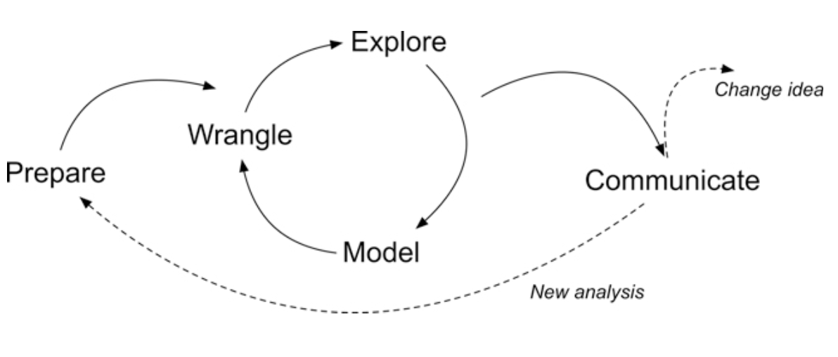
From Learning Analytics Goes to School (Krumm, Means, and Bienkowski 2018)

Speaker Notes:

Just as a quick refresher from our Learning Analytics Workflow Module, the workflow pictured here outlines a basic process intended to support researchers, practitioners, and data scientists prepare for a data-intensive analysis and communication of one’s findings. Different processes in this workflow as they relate to specific LA technique are highlighted in our code-along and presented in much greater detail in each case study.

If you’re interested in learning more about this workflow, I highly recommend the excellent book, Learning Analytics Goes to School, by Andrew Krumm, Barbara Means, and Marie Bienkowski.

Prepare

Guiding Research & Network Packages

Guiding Study

• Context
• Questions
• Data
• Findings

Revisiting early work in the field of sociometry, this study by Pittinsky and Carolan (2008) assesses the level of agreement between teacher perceptions and student reports of classroom friendships among middle school students.

Behavioral vs. Cognitive Classroom Friendships (Pittinsky and Carolan 2008)

The central question guiding this investigation was:

Do student reports agree with teacher perceptions when it comes to classroom friendship ties and with what consequences for commonly used social network measures?

• 1 teacher, 1 middle school, four classrooms

• Students given roster and asked to evaluate relationships with peers

• Choices included best friend, friend, know-like, know, know-dislike, strongly dislike, and do not know.

• Relations are valued (degrees of friendship, not just yes or no)

• Data are directed (friendship nominations were not presumed to be reciprocal).

• Teacher’s perceptions and students’ reports were statistically similar, 11–29% of possible ties did not match.

• Students reported significantly more reciprocated friendship ties than the teacher perceived.

• Observed level of agreement varied across classes and generally increased over time.

Speaker Notes:

Load Packages

• R Libraries
• Network Packages
• Your Turn

Let’s start by creating a new R script and loading the {tidyverse} package which we’ll use to import our network data files:

library(tidyverse)

# You may have to install this package if it is not listed in your packages pane.
# install.packages(tidyverse) 

Note: Tidyverse is actually a collection of R packages that share an underlying design philosophy, grammar, and data structures commonly referred to as “tidy data principles.” LASER uses the {tidyverse} extensively.

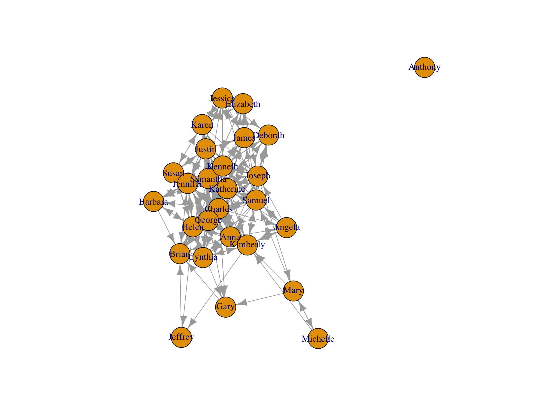
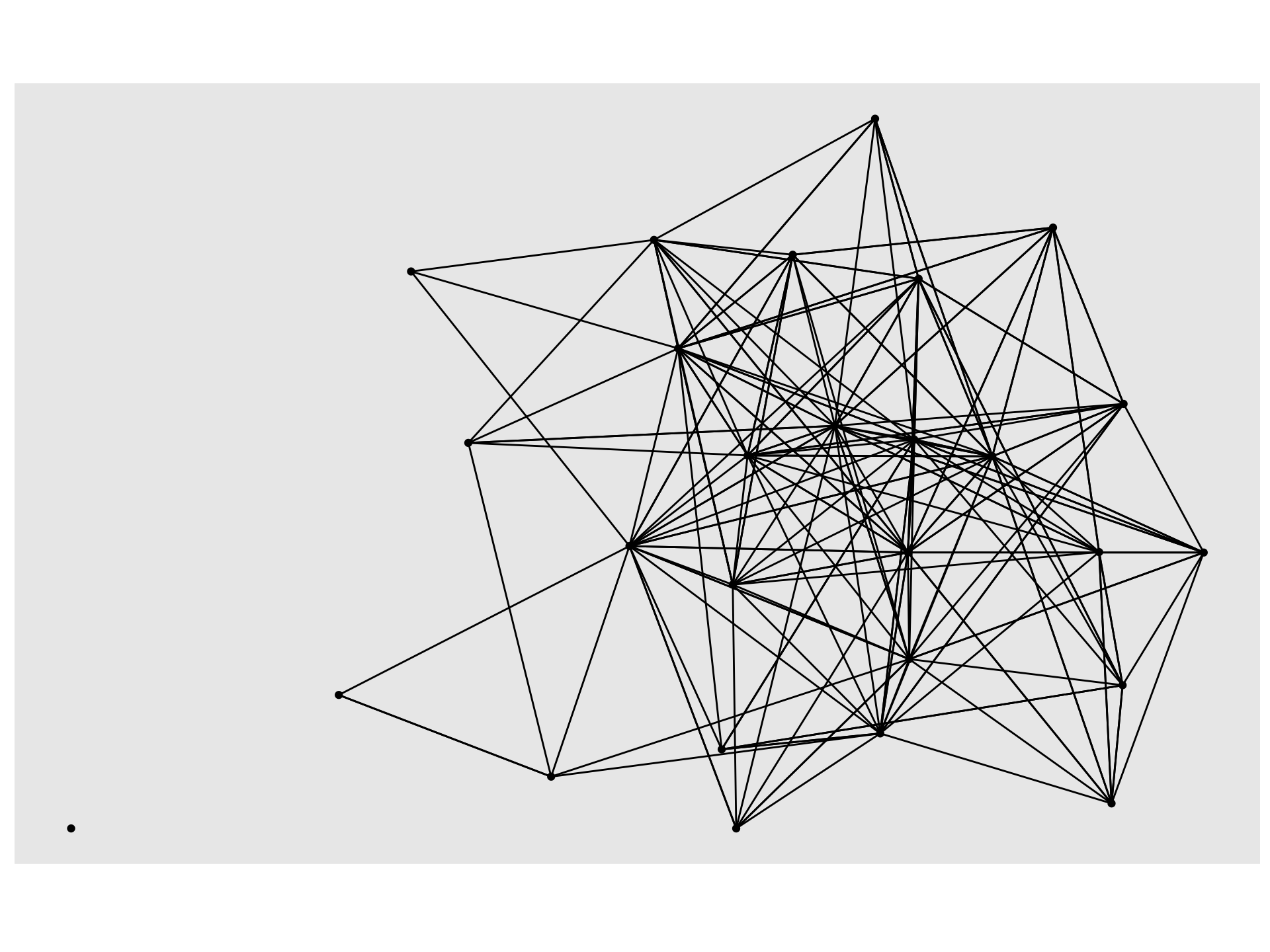
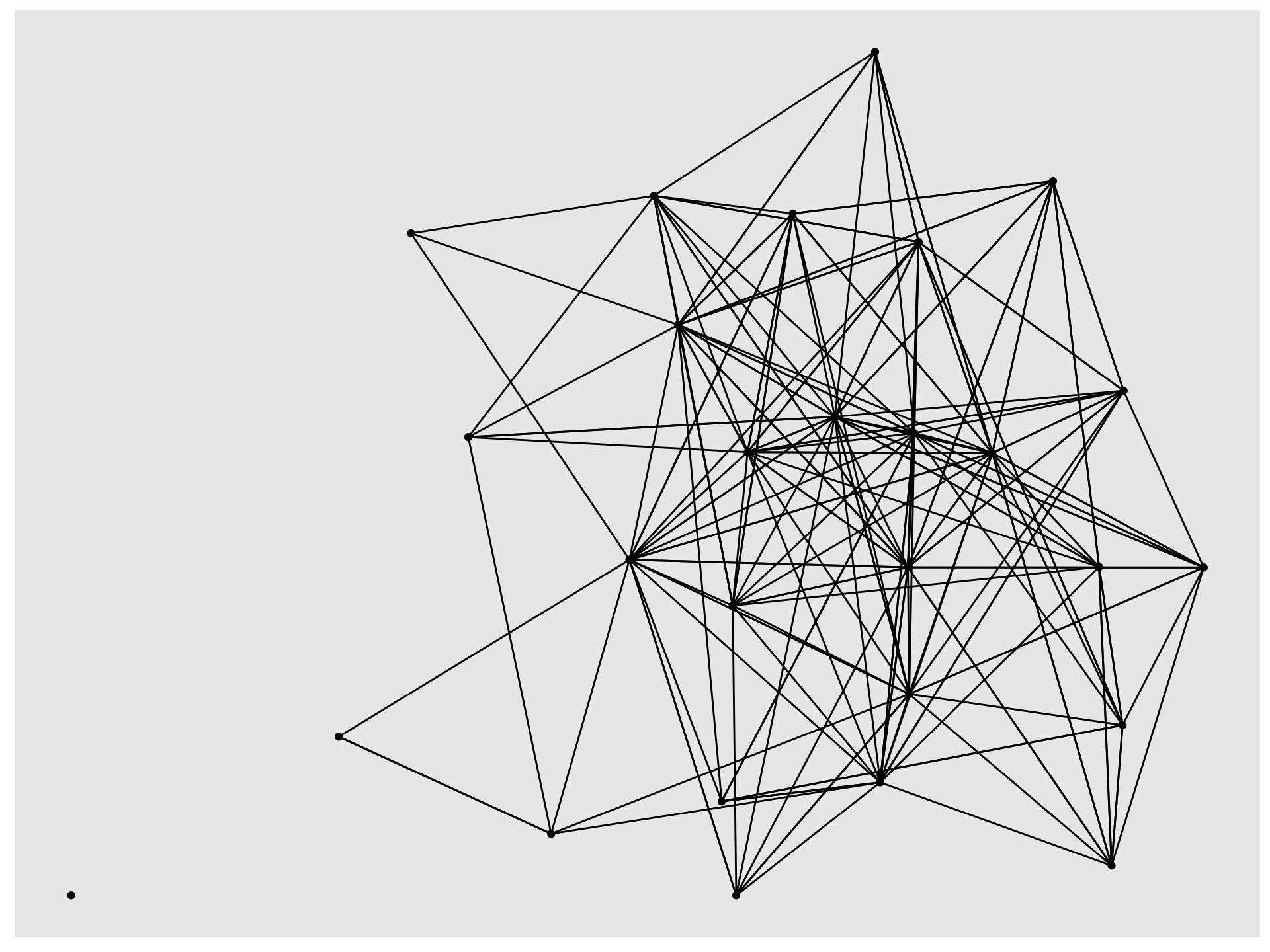
Data Management

tidygraph

Data Visualization

ggraph

Load the {tidygraph} and {ggraph} packages.

# YOUR CODE HERE
#
#

Wrangle

Intro to Network Data Structures

Network Data Structures

• Node-List
• Edge-List
• Adjacency Matrix
• Discuss

Consistent with typical data storage, node-lists often include:

• identifiers like name or ID

• demographic info (gender, age)

• socio-economic info (job, income)

• substantive info (grades, attendance)

id	gender	achievement
1	female	high
2	male	average
3	female	average
4	male	high
5	female	average
6	female	average

Radically different than typical data storage, edge-lists include:

• ego and an alter

• tie strength or frequency

• edge attributes (time, event, text)

from	to	weight
1	2	1
1	4	1
1	5	1
1	6	1
1	7	1
1	8	1

Also radically different, an adjacency matrix includes:

• column for each actor

• row for each actor

• a value indicating the presence/strength of a relation

	1	2	3	4	5	6	7
1	0	0	0	1	0	0	0
2	0	0	1	0	0	0	0
3	0	1	0	0	0	0	0
4	0	0	0	0	0	0	0
5	1	0	0	0	0	0	0
6	0	0	0	0	0	0	0
7	0	0	0	0	0	0	0

Take a look at one of the network datasets in the data folder under the Files Tab in RStudio and consider the following:

• What format is this data set stored as?

• If edge data, is it directed or undirected? Valued?

• If node data, does the file contain attribute data?

• What are some things you notice about this dataset?

• What questions do you have about this dataset?

Import Data

• Read Data
• Inspect Data
• Discuss

Let’s start by importing two .csv files that contain data about the nodes and the edges in our student friendship network:

student_nodes <- read_csv("lab-1/data/student-attributes.csv")

student_edges <- read_csv("lab-1/data/student-edgelist.csv")

Now let’s take a look at the data file we just imported using the View() function or another function of choice you may have learned previously:

View(student_edges)
View(student_nodes)

Think about the questions below and be prepared to share your response:

1. What do you think the rows and columns in each file represent?

2. What about the values in each cell represent?

3. What else do you notice about the data?

4. What questions do you have?

A Tidy Network

• tbl_graph( ) function
• View Network
• Output
• Discuss

Run the following code in your R script:

student_network <- tbl_graph(edges = student_edges,
                             nodes = student_nodes, 
                             directed = TRUE) 

The tbl_graph() function creates a special network data structure called a “tidy graph” that combines our nodes and edges into a single R object.

The benefits of a “tidy graph” is that it opens up the entire suite of tidyverse tools for manipulating and constructing network data and variables noted earlier.

Using your R script, type the name of network object we just created and run the code to produce the output on the next tab:

# ADD CODE BELOW
#
#

You should see an output that looks something like this:

# A tbl_graph: 27 nodes and 203 edges
#
# A directed simple graph with 2 components
#
# Node Data: 27 × 6 (active)
      id name      gender achievement gender_num achievement_num
   <dbl> <chr>     <chr>  <chr>            <dbl>           <dbl>
 1     1 Katherine female high                 1               1
 2     2 James     male   average              0               2
 3     3 Angela    female average              1               2
 4     4 Joseph    male   high                 0               1
 5     5 Samantha  female average              1               2
 6     6 Susan     female average              1               2
 7     7 Anna      female high                 1               1
 8     8 Kimberly  female average              1               2
 9     9 Helen     female high                 1               1
10    10 Samuel    male   low                  0               3
# ℹ 17 more rows
#
# Edge Data: 203 × 3
   from    to weight
  <int> <int>  <dbl>
1     1     2      1
2     1     4      1
3     1     5      1
# ℹ 200 more rows

Think about the questions below:

1. What is size of the student-reported friendship network?

2. What else do you notice about this network?

3. What questions do have about this network summary?

Explore

Making Simple and Sophisticated Sociograms

A Simple Sociogram

• plot()
• autograph()
• Arguments
• Discuss

Run the following code to make a simple sociogram:

plot(student_network)

The plot() function is base R’s simple but limited solution for plotting graphs.

The autograph() function is ggraph’s simple but limited solution for plotting sociograms.

autograph(student_network)

Both functions allow a small degree of customization, but are still limited.

autograph(student_network,
          node_label = name,
          node_colour = gender)

1. In what situations might these limited functions be useful?
2. When might they inappropriate to use?

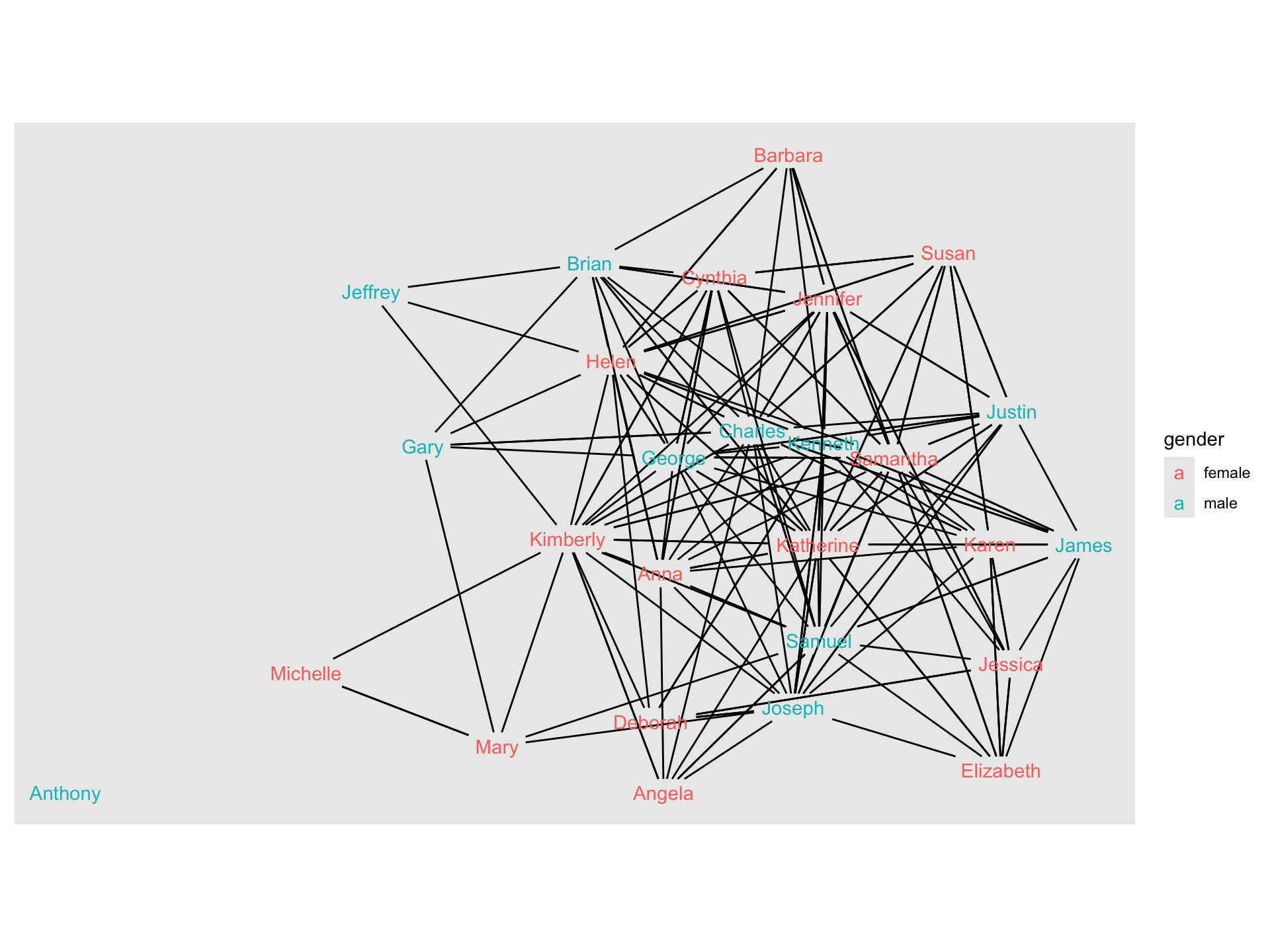
A Sophisticated Sociogram

• Set Graph
• “Add” Nodes
• “Add” Edges
• Polish
• Code

The ggraph() function is the first function required to build a sociogram. Try running this function on out student_network and see what happens:

ggraph(student_network)

This function serves two critical roles:

1. It takes care of setting up the plot object for the network specified.

2. It creates the layout based on algorithm provided.

Let’s “add” nodes to our sociogram using the + operator and the geom_node_point() function:

ggraph(student_network) + 
  geom_node_point() 

Both functions allow a small degree of customization, but are still limited.

ggraph(student_network) + 
  geom_node_point() + 
  geom_edge_link()

The {ggraph} packages allows for some very fairly sophisticated sociograms…

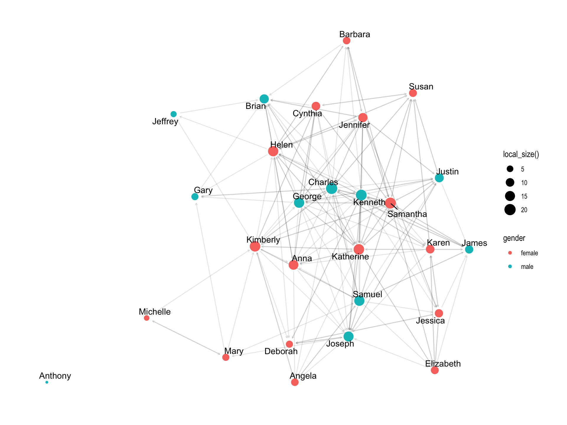
With a fair bit of coding:

ggraph(student_network, layout = "stress") + 
  geom_edge_link(arrow = arrow(length = unit(1, 'mm')), 
                 end_cap = circle(3, 'mm'),
                 start_cap = circle(3, 'mm'),
                 alpha = .1) +
  geom_node_point(aes(size = local_size(),
                      color = gender)) +
  geom_node_text(aes(label = name),
                 repel=TRUE) +
  theme_graph()

What’s Next?

• SNA Case Study: Who’s Friends with Who in Middle School?

• Guiding Study: Behavioral versus cognitive classroom friendship networks.

Acknowledgements

This work was supported by the National Science Foundation grants DRL-2025090 and DRL-2321128 (ECR:BCSER). Any opinions, findings, and conclusions expressed in this material are those of the authors and do not necessarily reflect the views of the National Science Foundation.

References

Krumm, Andrew, Barbara Means, and Marie Bienkowski. 2018. Learning Analytics Goes to School. Routledge. https://doi.org/10.4324/9781315650722.

Pittinsky, Matthew, and Brian V Carolan. 2008. “Behavioral Versus Cognitive Classroom Friendship Networks: Do Teacher Perceptions Agree with Student Reports?” Social Psychology of Education 11: 133–47. https://link.springer.com/content/pdf/10.1007/s11218-007-9046-7.pdf.