Model

LAW Module 3: A Code Along

Welcome to the LAW Code Along for Module 3

Modeling for educational researchers builds on insights from Exploratory Data Analysis (EDA) to develop predictive or explanatory models that guide decision-making and enhance learning outcomes.

This involves selecting appropriate models, preparing and transforming data, training and validating the models, and interpreting results. Effective modeling helps uncover key factors influencing educational success, allowing for targeted interventions and informed policy decisions.

Module Objectives

By the end of this module, learners will:

Understand the importance of modeling in the learning analytics workflow and how it helps quantify insights from data.

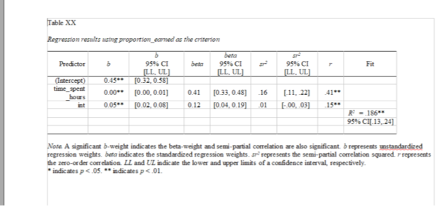
Create and interpret correlation matrices using the corrr package and create APA-formatted correlation tables using the apaTables package.

Fit and understand linear regression models to prepare for the case study.

In this module, we will focus on the practical aspects of modeling within the learning analytics workflow. By the end of this module, students will understand the importance of modeling and how it fits into the overall data analysis process. We will specifically cover the steps involved in creating and interpreting correlation matrices, fitting linear regression models, and validating model assumptions using R.

We’ll begin by learning how to create and interpret correlation matrices using the {corrr} package. This will help us identify and understand relationships between different variables in our data. We’ll also explore how to create APA-formatted correlation tables using the {apaTables} package, which are useful for formal reports and publications.

Next, we’ll apply various modeling techniques, starting with fitting linear regression models to predict academic achievement. We will also discuss the importance of validating model assumptions to ensure our models are robust and reliable. Additionally, we’ll use the summarize() function from the {dplyr} package to calculate summary statistics for our predictors, helping us to better understand our data and inform our modeling process. By the end of this module, students will have practical experience with these modeling techniques, enabling them to perform more advanced data analysis in their research.

Steps in the Modeling Process

The modeling phase is important for transforming the insights gained from Exploratory Data Analysis (EDA) into actionable predictions and explanations using statistical models.

Defining Objectives and Hypotheses:

The first step in modeling is to clearly define the objectives and hypotheses based on the insights gathered from EDA. This sets the direction for the modeling process and ensures that we are addressing the right questions.

Selecting Appropriate Models: Once we have our objectives, the next step is to select the appropriate models. This involves choosing the statistical or machine learning techniques that best fit our data and research questions. We will look at various models, such as linear regression, decision trees, and more complex algorithms.

Data Preparation and Feature Engineering:

Preparing the data is crucial for building effective models. This includes cleaning the data, handling missing values, and performing feature engineering to create new variables that better represent the underlying patterns in the data. We will use R to demonstrate these processes. Model Training and Validation:

After preparing the data, we move on to training our models. This involves fitting the models to our training data and using validation techniques to assess their performance. We will discuss the importance of splitting data into training and validation sets and using cross-validation to ensure robustness.

Interpreting Model Results:

Once the models are trained, we need to interpret the results. This step involves understanding the model outputs, such as coefficients in a regression model or feature importances in a tree-based model. We will learn how to extract meaningful insights from these results.

Assessing Model Performance:

Assessing model performance is critical to ensure that our models are accurate and reliable. We will use various metrics, such as accuracy, precision, recall, and RMSE, to evaluate the performance of our models and compare different models.

Refining and Tuning Models:

The final step in the modeling process is refining and tuning our models. This involves adjusting hyperparameters, experimenting with different algorithms, and performing feature selection to improve model performance. We will explore techniques for optimizing our models to achieve the best possible results.

The `corrr` Package

corrr allows you to run a correlation analysis between two variables.

#install corrr package if this is your first time
#install.packages("corrr")

# read in library
library(corrr) #<<
data_to_explore %>% 
  select(proportion_earned, time_spent_hours) %>%
  correlate() #<<

# A tibble: 2 × 3
  term              proportion_earned time_spent_hours
  <chr>                         <dbl>            <dbl>
1 proportion_earned            NA                0.438
2 time_spent_hours              0.438           NA

How can we interpret this?

Formatting `corrr` for APA

#install if this is your first time
install.packages("apaTables")

# read in apatables library
library(apaTables)

data_to_explore_subset <- data_to_explore %>% 
  select(time_spent_hours, proportion_earned, int)

apa.cor.table(data_to_explore_subset)#<<

Linear regression uses the lm() function.

lm(dependent ~ independent, data = "your data name")

Create a linear regression with time_spent_hours as the independent variable and proportion_earned as the dependent variable
Save as a new object model1
Inspect the data using summary()

model1 <- lm(proportion_earned ~ time_spent_hours, 
   data = data_to_explore)
summary(model1)


Call:
lm(formula = proportion_earned ~ time_spent_hours, data = data_to_explore)

Residuals:
    Min      1Q  Median      3Q     Max 
-64.671  -7.841   5.427  15.419  33.743 

Coefficients:
                 Estimate Std. Error t value Pr(>|t|)    
(Intercept)      62.43061    1.51073   41.33   <2e-16 ***
time_spent_hours  0.47921    0.04025   11.91   <2e-16 ***
---
Signif. codes:  0 '***' 0.001 '**' 0.01 '*' 0.05 '.' 0.1 ' ' 1

Residual standard error: 22.21 on 596 degrees of freedom
  (345 observations deleted due to missingness)
Multiple R-squared:  0.1921,    Adjusted R-squared:  0.1908 
F-statistic: 141.8 on 1 and 596 DF,  p-value: < 2.2e-16

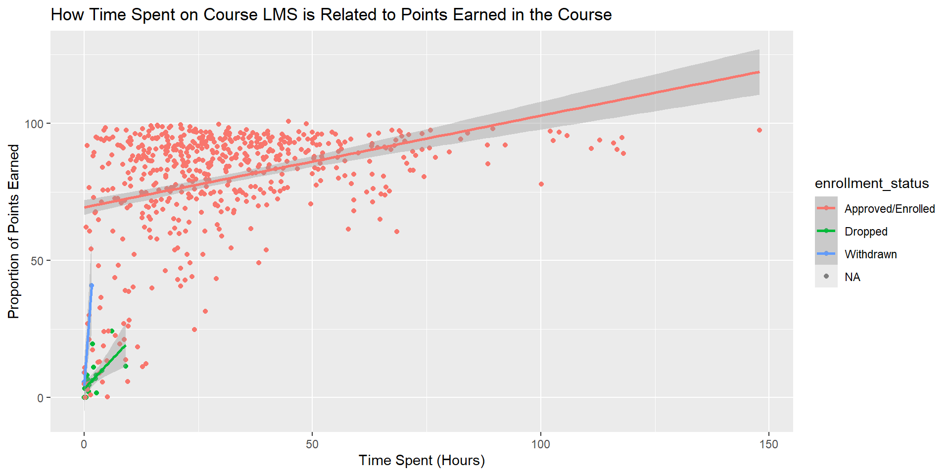
Create a ggplot viz for our model
Add + geom_smooth(method = "lm") after your geom_point

data_to_explore %>%
  ggplot(aes(x = time_spent_hours, 
             y = proportion_earned, 
             color = enrollment_status)) +
  geom_point() +
# add geom_smooth for lm
  geom_smooth(method = "lm")+
  labs(title="How Time Spent on Course LMS is Related to Points Earned in the Course", 
       x="Time Spent (Hours)",
       y = "Proportion of Points Earned")

MODEL TAB Quantify the insights using mathematical models. As highlighted in.Chapter 3 of Data Science in Education Using R, the Model step of the data science process entails “using statistical models, from simple to complex, to understand trends and patterns in the data.” The authors note that while descriptive statistics and data visualization during the Explore step can help us to identify patterns and relationships in our data, statistical models can be used to help us determine if relationships, patterns and trends are actually meaningful.

Correlation TAB

As highlighted in @macfadyen2010, scatter plots are a useful initial approach for identifying potential correlational trends between variables under investigation, but to further interrogate the significance of selected variables as indicators of student achievement, a simple correlation analysis of each variable with student final grade can be conducted.

There are two efficient ways to create correlation matrices, one that is best for internal use, and one that is best for inclusion in a manuscript. The {corrr} package provides a way to create a correlation matrix in a {tidyverse}-friendly way. Like for the {skimr} package, it can take as little as a line of code to create a correlation matrix. If not familiar, a correlation matrix is a table that presents how all of the variables are related to all of the other variables.

APA TABLE TAB While {corrr} is a nice package to quickly create a correlation matrix, you may wish to create one that is ready to be added directly to a dissertation or journal article. {apaTables} is great for creating more formal forms of output that can be added directly to an APA-formatted manuscript; it also has functionality for regression and other types of model output. It is not as friendly to {tidyverse} functions; first, we need to select only the variables we wish to correlate.

Then, we can use that subset of the variables as the argument to theapa.cor.table() function.

Run the following code to create a subset of the larger data_to_explore data frame with the variables you wish to correlate.

You will see a new Word document in your project folder called survey-cor-table.doc. Click on that and you’ll be prompted to download from your browser. It will look like the image on the right.

Linear Regression TAB At its basic we use the lm() function to regress one variable on another.

The code on the left estimates a model in which proportion_earned, the proportion of points students earned, is the dependent variable. It is predicted by one independent variable, int, students’ self-reported interest in science.

The code on the right regresses more than one variable on the dependent variable.

The following code estimates a model in which proportion_earned, the proportion of points students earned, is the dependent variable. It is predicted by one independent variable, int, students’ self-reported interest in science.

What’s Next?

Complete the Model part of the case study
Complete the Data Sources in Learning Analytics badge
Do essential readings for the next module