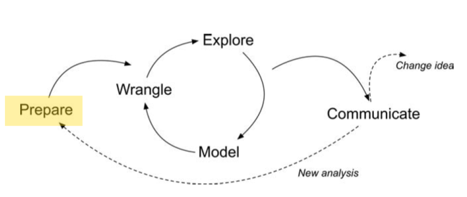
Prepare and Wrangle

LAW Module 1: A Code-A-long

Welcome to the LAW Code-a-long for Module 1

• Learning Analytics Workflow (LAW) is designed for those seeking an introductory understanding of learning analytics using basic R programming skills, particularly in the context of STEM education research.

• The following code-a-long is aimed at preparing you for the first section of the case study.

Prepare for a data-intensive analysis with clear and refined research questions with an understanding of where the data came from. For example, Krumm et al uses the example surrounding an activity system for which the technology was used.

You may ask yourself - Is it for instructional, reward or even a social collaborative context? Having that understanding will allow for more refined understanding when formulating guiding research questions for the analysis. Identify what gets collected and stored by technology is important for the development of the research question.

Here you may even refine your research question after having a better idea of where the data came from. The question may also be refined and redeveloped after you have started the data intensive analysis.

The Learning Analysis Cycle is not a linear process but rather a process of phases that can be moved around.

In this code-a-long session, we will concentrate on the “Prepare” phase of the Learning Analytics (LA) cycle. Before we delve into that, it’s essential to gain some context regarding the study that will inform our discussions today and over next three modules.

Module Objectives

By the end of this module:

• Know how to read in the data:
  • Learners will be able to identify and describe different types of learning environments, explaining their unique features and applications in educational research.

• Characteristics of Data:
  • Learners will gain proficiency in recognizing and categorizing various data formats commonly used in educational research by the end of this section.

Context of the Problem

Macfadyen, L. P., & Dawson, S. (2010). Mining LMS data to develop an “early warning system” for educators: A proof of concept. Computers & education, 54(2), 588-599.

• Explores specific online activities of students indicating their academic success.
• Focused on “early warning systems” in higher education.
• Research was extracted from course-based instructor tracking logs and the BB Vista production server.
• Data Sources
• A self-report survey assessing three aspects of students’ motivation
• Log-trace data, such as data output from the learning management system (LMS)
• Academic achievement data
• Discussion board data

Research Questions:

• Which LMS tracking data variables correlate significantly with student achievement?

• How accurately can measures of student online activity in an online course site predict student achievement in the course under study?

Installing and Loading Packages

• Install
• 👉 Your Turn ⤵
• Answer
• Load
• 👉 Your Turn ⤵
• Answer

• When you start a new session, you have to first install most packages to your development environment (RStudio)
• install.packages() downloads a package from a repository, typically the Comprehensive R Archive Network (CRAN) unless you say otherwise
• You only have to do this once per session
• When installing, red output text usually doesn’t necessarily mean there is a problem!

• Use install.packages() to install the tidyverse package

• Use quotations around the package name since it is identified as a string variable

# Install the tidyverse package
install.packages("tidyverse")

• Once you have a package installed, you load it into your session with library()

• Use library() to load the tidyverse package

• Since the package has been installed as an object in RStudio, don’t use quotations around the package name when loading it

# Load the tidyverse package
library(tidyverse)

PACKAGES-TAB

In order to read in data we must load packages that allow us to read data in, like we did in foundation lab 1. Although there are read-in capabilities with the utils package in base r, we are going to use a more modern approach. One of the packages in Tidyverse allows for reading in Comma delimiter files, or CSV.

Reminder if needed - this was discussed in foundation 1 R comes with several packages in base r when you start a session. Packages are a collection of objects, data sets around a theme or purpose. You may find a package whose objects are for the purpose of correlation, like in the cor package. Or you may find a package that has objects to produce better tables, like in the kable extra package. Or you may find a package that will help wrangling the data (processing it) easier than in Base R package. That is the package we are going to install here Tidyverse.

Tidyverse is a suite of packages that share a common philosophy and are designed to work together. Think Google products or Microsoft products. data importing, data wrangling and plotting.

Reading in Data with readr

• Common Arguments
• Delimiters
• 👉 Your Turn ⤵
• Answer

• file File to path

• col_names Uses the first row of raw data available as the column names if TRUE, creates placeholder column names if FALSE

• na Looks for text in the data to treat as non-applicable. Can be a list like c("", "na")

• skip Tells the function to “skip” ahead by reading at a given row of data.

• col_types Coerces columns to specific types of data. If NULL, the function guesses the type of each column, which is useful but not robust

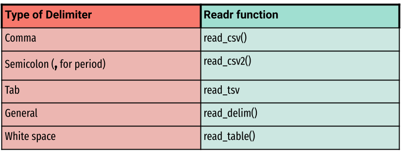
• Use read_csv() to read in sci-online.classes.csv

• This file is located in your data folder

#use read_csv function to read in sci-online-classes.csv rename object to online_classes
online_classes <- read_csv("data/sci-online-classes.csv")

#You can take a peek at the read in data with head()
knitr::kable(head(online_classes, n=5), format = 'html')

Common arguments that are included when you read in data are:

1. the file, we need to give a path to get the data. It should be in the working directory.

2. column names corresponds to variables on the first row. The first row of the input will be used as the column names, and will not be included in the data frame. If FALSE, column names will be generated automatically: X1, X2, X3 etc.

3. NA corresponds to missing values. commonly you will see capital NA but you may also see quotations or only a period depending on the original database (excel, SAS, STATA etc).

4. Skip functions allows you to skill to when your data starts.

5. col_types is not typically needed but good to know. R guesses what type of column types you have when it reads in the file using the default guess_max. This is convenient (and fast), but not robust. If the imputation fails, you’ll need to increase the guess_max or supply the correct types yourself.

readr is a quick way to read in comma-separated values (CSV) and tab-separated values (TSV)

• We read in from the path. My data is stored in a folder called data. I then use the assignment operator to save it as a new object called online-classes.
• (instructor is showing how to import from file) a quick way to see where your data file is stored is by clicking on the file under files and then import.
• Please note that we do NOT need to set working directory because we opened the projects folder. If we just click on the dataframe to open it it will not be connectd to the project.

Having a best practices way to set up your directory will help eleviate any confusion on data organization and location.

Other Data Types

• .xlsx
• 👉 Your Turn ⤵
• Answer
• .dta
• 👉 Your Turn ⤵
• Answer

• Excel files are proprietary to Microsoft but also very ubiquitous

• R solves this with readxl

• Load in the readxl package

• Read in csss_tweets.xlsx with the read_excel() function to a new object csss_tweets

• Inspect the object with head()

#Install and read in the readxl Package 
library(readxl)

#use read_excel() function to read in data/csss_tweets.xlsx
csss_tweets <- read_excel("data/csss_tweets.xlsx")#<<

#use head() function to read 
head(csss_tweets, n = 5)

# A tibble: 5 × 91
  user_id             status_id     created_at          screen_name text  source
  <chr>               <chr>         <dttm>              <chr>       <chr> <chr> 
1 1331246991762976769 136572200862… 2021-02-27 17:54:35 InnerSchol… "@We… Twitt…
2 1331246991762976769 136572187371… 2021-02-27 17:54:03 InnerSchol… "@Bo… Twitt…
3 1331246991762976769 136572178780… 2021-02-27 17:53:42 InnerSchol… "@Co… Twitt…
4 1331246991762976769 136572174606… 2021-02-27 17:53:32 InnerSchol… "@Co… Twitt…
5 1331246991762976769 136572164488… 2021-02-27 17:53:08 InnerSchol… "Ano… Twitt…
# ℹ 85 more variables: display_text_width <dbl>, reply_to_status_id <chr>,
#   reply_to_user_id <chr>, reply_to_screen_name <chr>, is_quote <lgl>,
#   is_retweet <lgl>, favorite_count <dbl>, retweet_count <dbl>,
#   quote_count <lgl>, reply_count <lgl>, hashtags <lgl>, symbols <lgl>,
#   urls_url <lgl>, urls_t.co <lgl>, urls_expanded_url <lgl>, media_url <lgl>,
#   media_t.co <lgl>, media_expanded_url <lgl>, media_type <lgl>,
#   ext_media_url <lgl>, ext_media_t.co <lgl>, ext_media_expanded_url <lgl>, …

• .dta files are used by statistical software like R, Python, Stata, and SAS

• They are accessed via haven

• Install and load in haven

• Read in GPA3.dta with the read_dta() function to a new object gpa_dt

• Inspect the object with head()

# Install and read in the haven function 
library(haven)

# Use read_dta() function to read in data/GPA3.dta
gpa_dt <- read_dta("data/GPA3.dta")
  
# Inspect the data
head(gpa_dt, n=3)

# A tibble: 3 × 23
   term   sat tothrs cumgpa season frstsem crsgpa verbmath trmgpa hssize hsrank
  <dbl> <dbl>  <dbl>  <dbl>  <dbl>   <dbl>  <dbl>    <dbl>  <dbl>  <dbl>  <dbl>
1     1   920     31   2.25      0       0   2.65    0.484   1.5      10      4
2     2   920     43   2.04      1       0   2.51    0.484   2.25     10      4
3     1   780     28   2.03      0       0   2.87    0.814   2.20    123    102
# ℹ 12 more variables: id <dbl>, spring <dbl>, female <dbl>, black <dbl>,
#   white <dbl>, ctrmgpa <dbl>, ctothrs <dbl>, ccrsgpa <dbl>, ccrspop <dbl>,
#   cseason <dbl>, hsperc <dbl>, football <dbl>

You can check what sheets are included in your excel file by calling it with the excel_sheets function. Then you can call only that sheet. Our data only includes one sheet so we do not really need to use this function, but it’s good to know.

Joining Data

• Mock Data
• Inner Join
• Left Join
• Right Join
• Full Join

Let’s create some mock data: One data frame for students, and one for scores.

# Create mock data
students <- data.frame(
  student_id = c(1, 2, 3, 4),
  name = c("Alice", "Bob", "Charlie", "David"),
  major = c("Math", "Physics", "Biology", "Computer Science")
)
students

  student_id    name            major
1          1   Alice             Math
2          2     Bob          Physics
3          3 Charlie          Biology
4          4   David Computer Science

scores <- data.frame(
  student_id = c(1, 2, 3, 5),
  score = c(85, 90, 75, 80)
)
scores

  student_id score
1          1    85
2          2    90
3          3    75
4          5    80

We are creating two mock data frames: students and scores. These data frames will help us demonstrate different types of joins in R.

library(tidyverse)
# Inner join: Returns rows that have matching values in both tables
inner_join_result <- inner_join(students, scores, by = "student_id")
inner_join_result

  student_id    name   major score
1          1   Alice    Math    85
2          2     Bob Physics    90
3          3 Charlie Biology    75

An inner join returns rows that have matching values in both tables. Only students present in both data frames are included in the result.

# Left join: Returns all rows from the left table, and the matched rows from the right table
# If there is no match, the result is NA
left_join_result <- left_join(students, scores, by = "student_id")
left_join_result

  student_id    name            major score
1          1   Alice             Math    85
2          2     Bob          Physics    90
3          3 Charlie          Biology    75
4          4   David Computer Science    NA

A left join returns all rows from the left table (students), and the matched rows from the right table (scores). If there is no match, the result is NA for the missing values.

# Right join: Returns all rows from the right table, and the matched rows from the left table. 
#If there is no match, the result is NA.
right_join_result <- right_join(students, scores, by = "student_id")
right_join_result

  student_id    name   major score
1          1   Alice    Math    85
2          2     Bob Physics    90
3          3 Charlie Biology    75
4          5    <NA>    <NA>    80

A right join returns all rows from the right table (scores), and the matched rows from the left table (students). If there is no match, the result is NA for the missing values.

# Full join: Returns all rows when there is a match in one of the tables. 
# If there is no match, the result is NA for the missing values.
full_join_result <- full_join(students, scores, by = "student_id")
full_join_result

  student_id    name            major score
1          1   Alice             Math    85
2          2     Bob          Physics    90
3          3 Charlie          Biology    75
4          4   David Computer Science    NA
5          5    <NA>             <NA>    80

❓ Why might you choose to use an inner join instead of a left join when analyzing student data alongside their scores and grades?

Question: Why might you choose to use an inner join instead of a left join when analyzing student data alongside their scores and grades?

Answer: You might choose to use an inner join instead of a left join when you only want to analyze the data for students who have both student information and corresponding scores. An inner join ensures that you are only working with complete data where there is a match in both tables, which can help avoid issues related to missing values and ensure the integrity of your analysis. This is particularly important when you need to perform calculations or statistical analyses that require complete data sets. By using an inner join, you ensure that the dataset you are working with is fully populated with the necessary information from both sources.

What’s Next?

• Explore the R Basics column of Posit Cloud’s Recipes
• Complete the Prepare and Wrangle part of the case study
• Complete the Foundations of Learning Analytics badge
• Do essential readings for the next module