We will focus on online science classes provided through a state-wide online virtual school and conduct an analysis that help product students’ performance in these online courses. This case study is guided by a foundational study in Learning Analytics that illustrates how analyses like these can be used develop an early warning system for educators to identify students at risk of failing and intervene before that happens.
Over the next labs we will dive into the Learning Analytics Workflow as follows:
Steps of Data-Intensive Research Workflow
Prepare: Prior to analysis, it’s critical to understand the context and data sources you’re working with so you can formulate useful and answerable questions. You’ll also need to become familiar with and load essential packages for analysis, and learn to load and view the data for analysis.
Wrangle: Wrangling data entails the work of manipulating, cleaning, transforming, and merging data. In Part 2 we focus on importing CSV files, tidying and joining our data.
Explore: In Part 3, we use basic data visualization and calculate some summary statistics to explore our data and see what insight it provides in response to our questions.
Model: After identifying variables that may be related to student performance through exploratory analysis, we’ll look at correlations and create some simple models of our data using linear regression.
Communicate: To wrap up our case study, we’ll develop our first “data product” and share our analyses and findings by creating our first web page using Markdown.
Change Idea: Having developed a webpage using Markdown, share your findings with the colleagues. The page will include interactive plots and a detailed explanation of the analysis process, serving as a case study for other educators in your school. Present your findings at a staff meeting, advocating for a broader adoption of data-driven strategies across curricula.
1. PREPARE (Module 1)
About the Study
This case study is guided by a well-cited publication from two authors that have made numerous contributions to the field of Learning Analytics over the years. This article is focused on “early warning systems” in higher education, and where adoption of learning management systems (LMS) like Moodle and Canvas gained a quicker foothold.
Previous research has indicated that universities and colleges could utilize Learning Management System (LMS) data to create reporting tools that identify students who are at risk and enable prompt pedagogical interventions. The present study validates and expands upon this idea by presenting data from an international research project that explores the specific online activities of students that reliably indicate their academic success. This paper confirms and extends this proposition by providing data from an international research project investigating which student online activities accurately predict academic achievement.
The data analyzed in this exploratory research was extracted from the course-based instructor tracking logs and the BB Vista production server.
Data collected on each student included ‘whole term’ counts for frequency of usage of course materials and tools supporting content delivery, engagement and discussion, assessment and administration/management. In addition, tracking data indicating total time spent on certain tool-based activities (assessments, assignments, total time online) offered a total measure of individual student time on task.
The authors used scatter plots for identifying potential relationships between variables under investigation, followed by a a simple correlation analysis of each variable to further interrogate the significance of selected variables as indicators of student achievement. Finally, a linear multiple regression analysis was conducted in order to develop a predictive model in which a student final grade was the continuous dependent variable.
Introduction to the Stakeholder
Name: Alex Johnson
Role: University Science Professor
Experience: 5 years teaching, enthusiastic about integrating technology in education
Goal: Alex aims to improve student engagement and performance in her online science classes.
Alex begins by understanding the importance of data analysis in identifying students who might need extra support. The cited foundational study motivates her to explore similar analyses to develop her own early warning system.
Load libraries
Remember libraries are also called packages. They are shareable collections of code that can contain functions, data, and/or documentation and extend the functionality of the coding language.
tidyverse is a collection of R packages designed for data manipulation, visualization, and analysis.
#Load Libraries below needed for analysislibrary(tidyverse)
Warning: package 'tidyverse' was built under R version 4.5.2
Warning: package 'tibble' was built under R version 4.5.2
Warning: package 'tidyr' was built under R version 4.5.2
Warning: package 'readr' was built under R version 4.5.2
Warning: package 'purrr' was built under R version 4.5.2
Warning: package 'dplyr' was built under R version 4.5.2
Warning: package 'stringr' was built under R version 4.5.2
Warning: package 'forcats' was built under R version 4.5.2
Warning: package 'lubridate' was built under R version 4.5.2
── Attaching core tidyverse packages ──────────────────────── tidyverse 2.0.0 ──
✔ dplyr     1.1.4     ✔ readr     2.1.6
✔ forcats   1.0.1     ✔ stringr   1.6.0
✔ ggplot2   4.0.2     ✔ tibble    3.3.1
✔ lubridate 1.9.4     ✔ tidyr     1.3.2
✔ purrr     1.2.1
── Conflicts ────────────────────────────────────────── tidyverse_conflicts() ──
✖ dplyr::filter() masks stats::filter()
✖ dplyr::lag()    masks stats::lag()
ℹ Use the conflicted package (<http://conflicted.r-lib.org/>) to force all conflicts to become errors
Data Source #1: Log Data
Log-trace data is data generated from our interactions with digital technologies, such as archived data from social media postings. In education, an increasingly common source of log-trace data is that generated from interactions with LMS and other digital tools.
The data we will use has already been “wrangled” quite a bit and is a summary type of log-trace data: the number of minutes students spent on the course. While this data type is fairly straightforward, there are even more complex sources of log-trace data out there (e.g., time stamps associated with when students started and stopped accessing the course).
Log Data Variables
Course Acronym Descriptions
Variable
Description
student_id
student’s id at institution
course_id
abbreviation for course, course number, semester
gender
male/female/NA
enrollment_reason
reason student decided to take the course
enrollment_status
approved/enrolled, dropped, withdrawn
time_spent
Time spent in hours for entire course
Acronym
Course Name
AnPhA
Anatomy
BioA
Biology
FrScA
Forensics
OcnA
Oceanography
PhysA
Physics
Data Source #2: Academic Achievement Data
Academic Achievement Data Variables
Variable
Description
total_points_possible
available points for the course
total_points_earned
points earned for the entire course
Data Source #3: Self-Report Survey
The third data source is a self-report survey. This was data collected before the start of the course. The survey included ten items, each corresponding to one of three motivation measures: interest, utility value, and perceived competence. These were chosen for their alignment with one way to think about students’ motivation, to what extent they expect to do well (corresponding to their perceived competence) and their value for what they are learning (corresponding to their interest and utility value).
Self-Report Survey Variables
Variable
Description
int
interest in science
tv
hours of TV watched
Q1 -Q10
survey questions
I think this course is an interesting subject. (Interest)
What I am learning in this class is relevant to my life. (Utility value)
I consider this topic to be one of my best subjects. (Perceived competence)
I am not interested in this course. (Interest—reverse coded)
I think I will like learning about this topic. (Interest)
I think what we are studying in this course is useful for me to know. (Utility value)
I don’t feel comfortable when it comes to answering questions in this area. (Perceived competence–reverse coded)
I think this subject is interesting. (Interest)
I find the content of this course to be personally meaningful. (Utility value)
I’ve always wanted to learn more about this subject. (Interest)
2. WRANGLE (Module 1)
Import data
We will need to load in and inspect each of the data frames that we will use for this lab. You will first read about the data frame and then learn how to load (or read in) the data frame into the quarto document.
time_spent
For our first data frame object, let’s use the read_csv() function from to import our log-data.csv file directly from our data folder.
We will save this data frame as an object called time_spent, to help us to quickly recollect what function it serves in this analysis. To do that, we need to enter this new name and assign its value using the <- operator.
👉 Your Turn⤵
You can run any code in a code block by pressing the green arrowhead in the top right corner. Try this one:
#load log-data file from data foldertime_spent <-read_csv("data/log-data.csv")
Rows: 716 Columns: 6
── Column specification ────────────────────────────────────────────────────────
Delimiter: ","
chr (4): course_id, gender, enrollment_reason, enrollment_status
dbl (2): student_id, time_spent

ℹ Use `spec()` to retrieve the full column specification for this data.
ℹ Specify the column types or set `show_col_types = FALSE` to quiet this message.
time_spent
# A tibble: 716 × 6
   student_id course_id    gender enrollment_reason enrollment_status time_spent
        <dbl> <chr>        <chr>  <chr>             <chr>                  <dbl>
 1      60186 AnPhA-S116-… M      Course Unavailab… Approved/Enrolled      2087.
 2      66693 AnPhA-S116-… M      Course Unavailab… Approved/Enrolled      2309.
 3      66811 AnPhA-S116-… F      Course Unavailab… Approved/Enrolled      5299.
 4      66862 AnPhA-S116-… F      Course Unavailab… Approved/Enrolled      1747.
 5      67508 AnPhA-S116-… F      Scheduling Confl… Approved/Enrolled      2668.
 6      70532 AnPhA-S116-… F      Learning Prefere… Approved/Enrolled      2938.
 7      77010 AnPhA-S116-… F      Learning Prefere… Approved/Enrolled      1533.
 8      85249 AnPhA-S116-… F      Course Unavailab… Approved/Enrolled      1210.
 9      85411 AnPhA-S116-… F      Scheduling Confl… Approved/Enrolled       473.
10      85583 AnPhA-S116-… F      Scheduling Confl… Approved/Enrolled      5532.
# ℹ 706 more rows
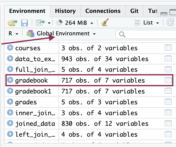
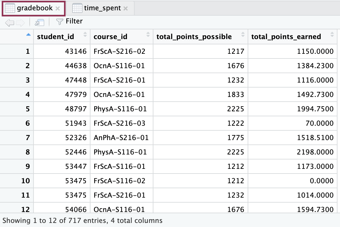
gradebook
Load the file gradebook-summary.csv from data folder and save the object as gradebook.
❗️In R, everything is an object. An object can be a simple value (like a number or a string), a complex structure (like a data frame or a list), or even a function or a model. For example, when you load a CSV file into R and store it in a variable, that variable is an object that contains your dataset.
A data set typically refers to a collection of data, often stored in a tabular format with rows and columns.
👉 Your Turn⤵
Use the same function as before to read in the gradebook-summary.csv file.
Make sure the output is assigned to a new object, this time called gradebook.
Press the green arrow head to run the code.
#load grade book data from data folder#(add code below)gradebook <-read_csv("data/gradebook-summary.csv",show_col_types =FALSE)
survey
Load the file survey.csv from data folder.
👉 Your Turn⤵
Use the same function as before to read in the gradebook-summary.csv file.
Make sure the output is assigned to a new object, this time called survey.
Press the green arrow head to run the code.
#load survey data from data folder#(add code below)survey <-read_csv("data/survey.csv",show_col_types =FALSE)
Inspect data
There are several ways you can look at data objects in R:
Simply typing the name of your object and running the code
time_spent
# A tibble: 716 × 6
   student_id course_id    gender enrollment_reason enrollment_status time_spent
        <dbl> <chr>        <chr>  <chr>             <chr>                  <dbl>
 1      60186 AnPhA-S116-… M      Course Unavailab… Approved/Enrolled      2087.
 2      66693 AnPhA-S116-… M      Course Unavailab… Approved/Enrolled      2309.
 3      66811 AnPhA-S116-… F      Course Unavailab… Approved/Enrolled      5299.
 4      66862 AnPhA-S116-… F      Course Unavailab… Approved/Enrolled      1747.
 5      67508 AnPhA-S116-… F      Scheduling Confl… Approved/Enrolled      2668.
 6      70532 AnPhA-S116-… F      Learning Prefere… Approved/Enrolled      2938.
 7      77010 AnPhA-S116-… F      Learning Prefere… Approved/Enrolled      1533.
 8      85249 AnPhA-S116-… F      Course Unavailab… Approved/Enrolled      1210.
 9      85411 AnPhA-S116-… F      Scheduling Confl… Approved/Enrolled       473.
10      85583 AnPhA-S116-… F      Scheduling Confl… Approved/Enrolled      5532.
# ℹ 706 more rows
# A tibble: 662 × 26
      q9 percomp    q2 post_uv    tv course_ID        q3 post_int    q1
   <dbl>   <dbl> <dbl>   <dbl> <dbl> <chr>         <dbl>    <dbl> <dbl>
 1     3     4       4   NA     3.86 FrScA-S216-02     4    NA        4
 2     3     3       2   NA     3.57 OcnA-S116-01      2    NA        4
 3     3     3       3   NA     3.71 FrScA-S216-01     3    NA        5
 4     4     2.5     3   NA     3.86 OcnA-S216-01      2    NA        4
 5     3     3.5     4   NA     3.71 PhysA-S116-01     3    NA        4
 6     4     3.5     4   NA     3.71 FrScA-S216-03     3    NA        4
 7     4     3       4   NA     4    AnPhA-S216-01     4    NA        4
 8     3     3       4    3.67  4    PhysA-S116-01     3     3.5      4
 9     2     3       2    2     3    FrScA-S116-01     3     3.75     5
10     3     4       4   NA     4.14 FrScA-S216-01     4    NA        5
# ℹ 652 more rows
# ℹ 17 more variables: date.y <dttm>, val <dbl>, subject <chr>, q7 <dbl>,
#   int <dbl>, q5 <dbl>, semester <chr>, q4 <dbl>, post_tv <dbl>, q8 <dbl>,
#   q6 <dbl>, student_ID <chr>, section <chr>, post_percomp <dbl>,
#   date.x <dttm>, date <dttm>, q10 <dbl>
👉 Your Turn⤵
Inspect the three datasets we loaded and answer the questions:
❓ What do you notice or wonder about?
[YOUR RESPONSE HERE]
❓ How many observations do you see?
[YOUR RESPONSE HERE]
❓ How many variables are there?
[YOUR RESPONSE HERE]
❓ What do you notice about the variable classes?
[YOUR RESPONSE HERE]
Tidy data
time_spent
Use separate() function from tidyr
Using separate(), we will turn the course_id variable in time_spent into three different variables: The course subject, semester, and section.
The c() function in R is used used to combine or concatenate its argument. You can use it to get the output by giving parameters inside the function.
#separate variable to individual subject, semester and sectiontime_spent %>%separate(course_id,c("subject", "semester", "section"))
# A tibble: 716 × 8
   student_id subject semester section gender enrollment_reason
        <dbl> <chr>   <chr>    <chr>   <chr>  <chr>
 1      60186 AnPhA   S116     01      M      Course Unavailable at Local School
 2      66693 AnPhA   S116     01      M      Course Unavailable at Local School
 3      66811 AnPhA   S116     01      F      Course Unavailable at Local School
 4      66862 AnPhA   S116     01      F      Course Unavailable at Local School
 5      67508 AnPhA   S116     01      F      Scheduling Conflict
 6      70532 AnPhA   S116     01      F      Learning Preference of the Student
 7      77010 AnPhA   S116     01      F      Learning Preference of the Student
 8      85249 AnPhA   S116     01      F      Course Unavailable at Local School
 9      85411 AnPhA   S116     01      F      Scheduling Conflict
10      85583 AnPhA   S116     01      F      Scheduling Conflict
# ℹ 706 more rows
# ℹ 2 more variables: enrollment_status <chr>, time_spent <dbl>
#inspecttime_spent
# A tibble: 716 × 6
   student_id course_id    gender enrollment_reason enrollment_status time_spent
        <dbl> <chr>        <chr>  <chr>             <chr>                  <dbl>
 1      60186 AnPhA-S116-… M      Course Unavailab… Approved/Enrolled      2087.
 2      66693 AnPhA-S116-… M      Course Unavailab… Approved/Enrolled      2309.
 3      66811 AnPhA-S116-… F      Course Unavailab… Approved/Enrolled      5299.
 4      66862 AnPhA-S116-… F      Course Unavailab… Approved/Enrolled      1747.
 5      67508 AnPhA-S116-… F      Scheduling Confl… Approved/Enrolled      2668.
 6      70532 AnPhA-S116-… F      Learning Prefere… Approved/Enrolled      2938.
 7      77010 AnPhA-S116-… F      Learning Prefere… Approved/Enrolled      1533.
 8      85249 AnPhA-S116-… F      Course Unavailab… Approved/Enrolled      1210.
 9      85411 AnPhA-S116-… F      Scheduling Confl… Approved/Enrolled       473.
10      85583 AnPhA-S116-… F      Scheduling Confl… Approved/Enrolled      5532.
# ℹ 706 more rows
Make sure to save it to the time_spent object. Saving an object is accomplished by using an assignment operator, which looks kind of like an arrow <- It is generally best practice to put the assigned object on the left, at the beginning of the code.
time_spent <- time_spent %>%#save function output to existing object separate(course_id,c("subject", "semester", "section"))#inspecttime_spent
# A tibble: 716 × 8
   student_id subject semester section gender enrollment_reason
        <dbl> <chr>   <chr>    <chr>   <chr>  <chr>
 1      60186 AnPhA   S116     01      M      Course Unavailable at Local School
 2      66693 AnPhA   S116     01      M      Course Unavailable at Local School
 3      66811 AnPhA   S116     01      F      Course Unavailable at Local School
 4      66862 AnPhA   S116     01      F      Course Unavailable at Local School
 5      67508 AnPhA   S116     01      F      Scheduling Conflict
 6      70532 AnPhA   S116     01      F      Learning Preference of the Student
 7      77010 AnPhA   S116     01      F      Learning Preference of the Student
 8      85249 AnPhA   S116     01      F      Course Unavailable at Local School
 9      85411 AnPhA   S116     01      F      Scheduling Conflict
10      85583 AnPhA   S116     01      F      Scheduling Conflict
# ℹ 706 more rows
# ℹ 2 more variables: enrollment_status <chr>, time_spent <dbl>
Use mutate() function from dplyr
As you can see from the dataset, time_spent variable is not set in hours. Let’s change that.
In R, you can create new variables in a dataset (data frame or tibble) using mutate(), which allows you to add new columns to your data frame or modify existing ones.
#mutate minutes to hours on time spent and save as new variable.time_spent <- time_spent %>%mutate(time_spent_hours = time_spent /60)#inspect time_spent
# A tibble: 716 × 9
   student_id subject semester section gender enrollment_reason
        <dbl> <chr>   <chr>    <chr>   <chr>  <chr>
 1      60186 AnPhA   S116     01      M      Course Unavailable at Local School
 2      66693 AnPhA   S116     01      M      Course Unavailable at Local School
 3      66811 AnPhA   S116     01      F      Course Unavailable at Local School
 4      66862 AnPhA   S116     01      F      Course Unavailable at Local School
 5      67508 AnPhA   S116     01      F      Scheduling Conflict
 6      70532 AnPhA   S116     01      F      Learning Preference of the Student
 7      77010 AnPhA   S116     01      F      Learning Preference of the Student
 8      85249 AnPhA   S116     01      F      Course Unavailable at Local School
 9      85411 AnPhA   S116     01      F      Scheduling Conflict
10      85583 AnPhA   S116     01      F      Scheduling Conflict
# ℹ 706 more rows
# ℹ 3 more variables: enrollment_status <chr>, time_spent <dbl>,
#   time_spent_hours <dbl>
gradebook
Use separate() function from tidyr
Now, we will work on the gradebook dataset. Like the previous dataset, we will separate the course_id variable again.
👉 Your Turn⤵
Use the pipe operator to separate course_id variable (like we just did in time_spent).
Run the code.
#separate the course_id variable and save to 'gradebook' object#YOUR CODE HEREgradebook <- gradebook %>%separate(course_id,c("subject", "semester", "section"))#inspect#YOUR CODE HEREgradebook
As you can see in gradebook, it is hard to see total_points_earned as a proportion. We can use mutate() to make it a percentage.
👉 Your Turn⤵
Take total_points_earned divide by total_points_possible and multiply by 100. Save this as proportion_earned.
Run the code.
# Mutate to a proportion_earned, take 'total points earned' divide by 'total points possible.' Save as a new variable proportion_earned.gradebook <- gradebook %>%mutate(proportion_earned = (total_points_earned /total_points_possible) *100)#YOUR CODE HERE#inspect datagradebook
Let’s process our data. First though, take a quick look again by typing survey into the console or using a preferred viewing method to take a look at the data.
❓ Does it appear to be the correct file? What do the variables seem to be about? What wrangling steps do we need to take? Taking a quick peak at the data helps us to begin to formulate answers to these and is an important step in any data analysis, especially as we prepare for what we are going to do.
💡 Look at the variable names. Add one or more of the things you notice or wonder about the data here:
[YOUR RESPONSES HERE]
[YOUR RESPONSES HERE]
You may have noticed that student_ID is not formatted exactly the same as student_id in our other files. This is important because in the next section when we “join,” or merge, our data files, these variables will need to have identical names.
Use the janitor package
Fortunately the {janitor} package has simple functions for examining and cleaning dirty data. It was built with beginning and intermediate R users in mind and is optimized for user-friendliness. There is also a handy function called clean_names() in the {janitor} package for standardizing variable names.
👉 Your Turn⤵
First, add the janitor package using the library() function.
# load janitor library to clean variable names that do not match#YOUR CODE HERElibrary(janitor)
Clean the columns by adding the survey object to the clean_names() function and saving it to thesurvey object.
Inspect the data.
Run the code.
#clean columns of the survey data and save to survey object#(add code below - some code is given to you)survey <-clean_names(survey)#inspect data to check for consistency with other data#(add code below)survey
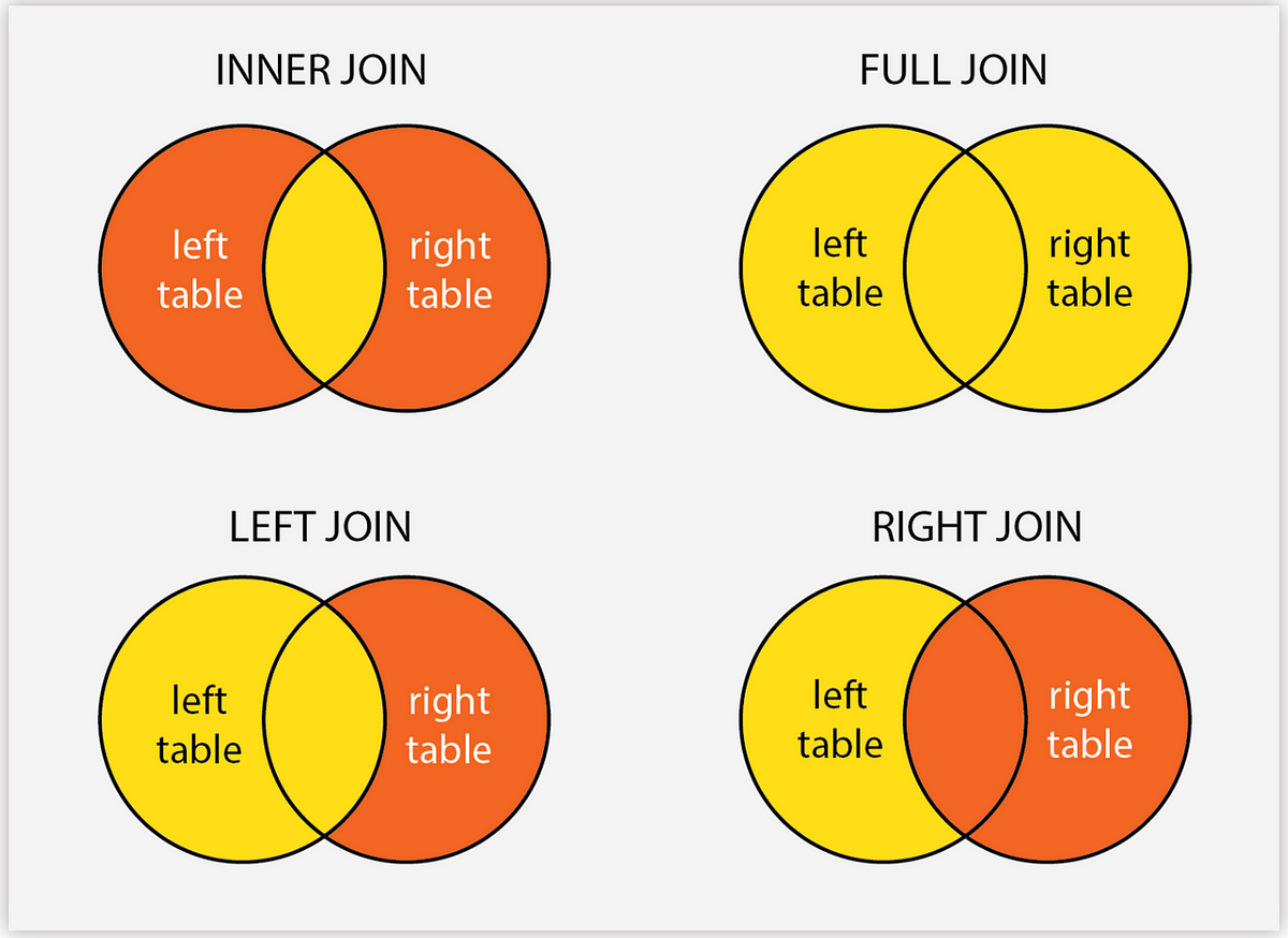
A full_join() is best for our need to combine information from all three datasets. full_join() returns all of the records in a new table, whether it matches on either the left or right tables. If the table rows match, then a join will be executed, otherwise it will return NULL in places where a matching row does not exist.
Similar to what we learned in the code-a-long, we will combine the gradebook and time_spent datasets. We first should identify the variables (column names) to combine. In this case, we will use the following:
student_id
subject
semester
section
#use single join to join data sets by student_id, subject, semester and section.joined_data <-full_join(gradebook, time_spent, by =c("student_id", "subject", "semester", "section"))#inspect joined_data
As you can see, we have the new dataset joined_data. Those 12 variables came from the gradebook and time_spent datasets.
Join the survey and joined_data data sets
👉 Your Turn⤵
Use the full_join() function to join joined_data with survey, identifying the following variables:
student_id
subject
semester
section
Save to a new object called data_to_explore.
Inspect the data.
Run the code.
#use join to join data sets by student_id, subject, semester and section.#(add code below - some code has been added for you)data_to_explore <-full_join(survey, joined_data, by =c("student_id", "subject", "semester", "section"))#inspectdata_to_explore
DON’T PANIC if you are getting an error - read below!!
These datasets cannot be joined because the class (data type) of student_id is different than joined_data.
👉Your Turn⤵
❓ Check out what class student_id is in joined_data compared to survey. What do you notice? (Hint: think about the class())
[YOUR ANSWER HERE]
Use as.character()
We need to change joined_data’s student_id variable into a character class to match that of survey using mutate().
👉 Your Turn⤵
Use the mutate() function and as.character() function to change student_id variable from numeric to character class.
Save the new value to the student_id variable.
Run the code.
#mutate to change variable class from double or numeric to character#(add code below - some code has been already added)joined_data <- joined_data %>%mutate(student_id =as.character(student_id))#inspectjoined_data
Use the full_join() function to join joined_data with survey, identifying the following variables:
student_id
subject
semester
section
Save to a new object called data_to_explore.
Inspect the data.
Run the code.
#try again to together the grade_book and log_wrangled#(add code below - some code has been already added)data_to_explore <-full_join(survey, joined_data, by =c("student_id", "subject", "semester", "section"))#inspectdata_to_explore
Let’s also transform the subject names to a more convenient format:
data_to_explore <- data_to_explore %>%mutate(subject =case_when( subject =="AnPhA"~"Anatomy", subject =="BioA"~"Biology", subject =="FrScA"~"Forensics", subject =="OcnA"~"Oceanography", subject =="PhysA"~"Physics",TRUE~ subject #This line keeps the original value if none of the conditions above are met ))data_to_explore
Alex follows the steps to load and wrangle data, reflecting on how each step can provide insights into her students’ engagement levels. She is particularly interested in understanding patterns in the time students spend on different course materials and how these patterns correlate with their performance.
Filter and sort data
Use filter() from the dplyr package
We can identify students at risk of failing the course using the filter function looking at students below 70:
#Filter students with lower gradesat_risk_students <- data_to_explore %>%filter(proportion_earned<70)#Print the at-risk studentsat_risk_students
Think what other factors are important to identify students at risk. Run your code and analyze the results:
#YOUR CODE HERE:
Export and back up data
Now let’s write the file to our data folder using write_csv() to save for later or download.
# add the function to write data to file to use laterwrite_csv(data_to_explore, "module_1/data/data_to_explore.csv")
Check the data folder to confirm the location of your new file.
🛑 Stop here! Congratulations, you finished the first part of the case study.
3. EXPLORE (Module 2)
Exploratory Data Analysis
Use the skimr package
We’ve already wrangled our data, but let’s look at the data frame to make sure it is still correct. A quick way to look at the data frame is with skimr.
This output is best for internal use. This is because the output is rich, but not well-suited to exporting to a table that you add, for instance, to a Google Docs or Microsoft Word manuscript.
Of course, these values can be entered manually into a table, but we’ll also discuss ways later on to create tables that are ready, or nearly-ready-to be added directly to manuscripts.
👉 Your Turn⤵
Load skimr with the correct function.
#load library by adding skimr as the package name#(add code below)library(skimr)
Normally you would do this above, but we want to make sure you know which packages are used with the new functions.
Next, use skim() to view data_to_explore.
#skim the data by adding the skim function in front of the data#(add code below)skim(data_to_explore)
Data summary
Name
data_to_explore
Number of rows
943
Number of columns
34
_______________________
Column type frequency:
character
8
numeric
23
POSIXct
3
________________________
Group variables
None
Variable type: character
skim_variable
n_missing
complete_rate
min
max
empty
n_unique
whitespace
student_id
0
1.00
2
6
0
879
0
course_id
281
0.70
12
13
0
36
0
subject
0
1.00
7
12
0
5
0
semester
0
1.00
4
4
0
4
0
section
0
1.00
2
2
0
4
0
gender
227
0.76
1
1
0
2
0
enrollment_reason
227
0.76
5
34
0
5
0
enrollment_status
227
0.76
7
17
0
3
0
Variable type: numeric
skim_variable
n_missing
complete_rate
mean
sd
p0
p25
p50
p75
p100
hist
int
293
0.69
4.30
0.60
1.80
4.00
4.40
4.80
5.00
▁▁▂▆▇
val
287
0.70
3.75
0.75
1.00
3.33
3.67
4.33
5.00
▁▁▆▇▆
percomp
288
0.69
3.64
0.69
1.50
3.00
3.50
4.00
5.00
▁▁▇▃▃
tv
292
0.69
4.07
0.59
1.00
3.71
4.12
4.46
5.00
▁▁▂▇▇
q1
285
0.70
4.34
0.66
1.00
4.00
4.00
5.00
5.00
▁▁▁▇▇
q2
285
0.70
3.66
0.93
1.00
3.00
4.00
4.00
5.00
▁▂▆▇▃
q3
286
0.70
3.31
0.85
1.00
3.00
3.00
4.00
5.00
▁▂▇▅▂
q4
289
0.69
4.35
0.80
1.00
4.00
5.00
5.00
5.00
▁▁▁▆▇
q5
286
0.70
4.28
0.69
1.00
4.00
4.00
5.00
5.00
▁▁▁▇▆
q6
285
0.70
4.05
0.80
1.00
4.00
4.00
5.00
5.00
▁▁▃▇▅
q7
286
0.70
3.96
0.85
1.00
3.00
4.00
5.00
5.00
▁▁▅▇▆
q8
286
0.70
4.35
0.65
1.00
4.00
4.00
5.00
5.00
▁▁▁▇▇
q9
286
0.70
3.55
0.92
1.00
3.00
4.00
4.00
5.00
▁▂▇▇▃
q10
285
0.70
4.17
0.87
1.00
4.00
4.00
5.00
5.00
▁▁▃▇▇
post_int
848
0.10
3.88
0.94
1.00
3.50
4.00
4.50
5.00
▁▁▃▇▇
post_uv
848
0.10
3.48
0.99
1.00
3.00
3.67
4.00
5.00
▂▂▅▇▅
post_tv
848
0.10
3.71
0.90
1.00
3.29
3.86
4.29
5.00
▁▂▃▇▆
post_percomp
848
0.10
3.47
0.88
1.00
3.00
3.50
4.00
5.00
▁▂▂▇▂
total_points_possible
226
0.76
1619.55
387.12
1212.00
1217.00
1676.00
1791.00
2425.00
▇▂▆▁▃
total_points_earned
226
0.76
1229.98
510.64
0.00
1002.50
1177.13
1572.45
2413.50
▂▂▇▅▂
proportion_earned
226
0.76
76.23
25.20
0.00
72.36
85.59
92.29
100.74
▁▁▁▃▇
time_spent
232
0.75
1828.80
1363.13
0.45
895.57
1559.97
2423.94
8870.88
▇▅▁▁▁
time_spent_hours
232
0.75
30.48
22.72
0.01
14.93
26.00
40.40
147.85
▇▅▁▁▁
Variable type: POSIXct
skim_variable
n_missing
complete_rate
min
max
median
n_unique
date_x
393
0.58
2015-09-02 15:40:00
2016-05-24 15:53:00
2015-10-01 15:57:30
536
date_y
848
0.10
2015-09-02 15:31:00
2016-01-22 15:43:00
2016-01-04 13:25:00
95
date
834
0.12
2017-01-23 13:14:00
2017-02-13 13:00:00
2017-01-25 18:43:00
107
Finally, use the group_by() function (from dplyr) on the subject variable, then the skim() function (from skimr).
data_to_explore %>%group_by(subject)%>%skim()
Data summary
Name
Piped data
Number of rows
943
Number of columns
34
_______________________
Column type frequency:
character
7
numeric
23
POSIXct
3
________________________
Group variables
subject
Variable type: character
skim_variable
subject
n_missing
complete_rate
min
max
empty
n_unique
whitespace
student_id
Anatomy
0
1.00
2
6
0
207
0
student_id
Biology
0
1.00
3
6
0
47
0
student_id
Forensics
0
1.00
2
6
0
414
0
student_id
Oceanography
0
1.00
2
6
0
171
0
student_id
Physics
0
1.00
3
6
0
74
0
course_id
Anatomy
58
0.72
13
13
0
7
0
course_id
Biology
7
0.86
12
12
0
4
0
course_id
Forensics
150
0.66
13
13
0
12
0
course_id
Oceanography
55
0.69
12
12
0
9
0
course_id
Physics
11
0.85
13
13
0
4
0
semester
Anatomy
0
1.00
4
4
0
4
0
semester
Biology
0
1.00
4
4
0
4
0
semester
Forensics
0
1.00
4
4
0
4
0
semester
Oceanography
0
1.00
4
4
0
4
0
semester
Physics
0
1.00
4
4
0
4
0
section
Anatomy
0
1.00
2
2
0
2
0
section
Biology
0
1.00
2
2
0
1
0
section
Forensics
0
1.00
2
2
0
4
0
section
Oceanography
0
1.00
2
2
0
3
0
section
Physics
0
1.00
2
2
0
1
0
gender
Anatomy
45
0.79
1
1
0
2
0
gender
Biology
4
0.92
1
1
0
2
0
gender
Forensics
130
0.70
1
1
0
2
0
gender
Oceanography
42
0.76
1
1
0
2
0
gender
Physics
6
0.92
1
1
0
2
0
enrollment_reason
Anatomy
45
0.79
5
34
0
4
0
enrollment_reason
Biology
4
0.92
5
34
0
5
0
enrollment_reason
Forensics
130
0.70
5
34
0
5
0
enrollment_reason
Oceanography
42
0.76
5
34
0
5
0
enrollment_reason
Physics
6
0.92
5
34
0
4
0
enrollment_status
Anatomy
45
0.79
7
17
0
2
0
enrollment_status
Biology
4
0.92
7
17
0
3
0
enrollment_status
Forensics
130
0.70
7
17
0
3
0
enrollment_status
Oceanography
42
0.76
7
17
0
3
0
enrollment_status
Physics
6
0.92
7
17
0
2
0
Variable type: numeric
skim_variable
subject
n_missing
complete_rate
mean
sd
p0
p25
p50
p75
p100
hist
int
Anatomy
62
0.70
4.42
0.57
1.80
4.00
4.40
5.00
5.00
▁▁▁▅▇
int
Biology
9
0.82
3.69
0.63
2.40
3.35
3.80
4.00
5.00
▂▆▇▆▂
int
Forensics
154
0.65
4.42
0.52
2.60
4.00
4.40
5.00
5.00
▁▁▃▃▇
int
Oceanography
56
0.68
4.24
0.58
2.20
4.00
4.20
4.60
5.00
▁▁▂▇▆
int
Physics
12
0.84
4.00
0.65
2.20
3.60
4.00
4.40
5.00
▁▂▆▇▅
val
Anatomy
59
0.72
4.29
0.62
1.00
4.00
4.33
4.67
5.00
▁▁▁▅▇
val
Biology
7
0.86
3.50
0.58
2.67
3.00
3.33
3.67
5.00
▆▆▇▁▂
val
Forensics
155
0.64
3.53
0.72
1.67
3.00
3.67
4.00
5.00
▂▅▇▅▂
val
Oceanography
55
0.69
3.62
0.77
1.00
3.00
3.67
4.00
5.00
▁▁▅▇▃
val
Physics
11
0.85
3.89
0.56
2.00
3.67
4.00
4.33
5.00
▁▁▇▇▃
percomp
Anatomy
61
0.71
3.80
0.67
2.00
3.50
4.00
4.50
5.00
▂▃▇▆▇
percomp
Biology
8
0.84
3.34
0.75
2.00
3.00
3.00
4.00
5.00
▅▇▃▇▂
percomp
Forensics
152
0.65
3.64
0.63
1.50
3.00
3.50
4.00
5.00
▁▁▇▅▃
percomp
Oceanography
56
0.68
3.57
0.67
2.00
3.00
3.50
4.00
5.00
▂▇▆▅▅
percomp
Physics
11
0.85
3.56
0.84
2.00
3.00
3.50
4.00
5.00
▅▅▇▅▇
tv
Anatomy
60
0.71
4.35
0.57
1.00
4.00
4.43
4.83
5.00
▁▁▁▅▇
tv
Biology
9
0.82
3.61
0.56
2.29
3.14
3.57
3.86
5.00
▁▃▇▂▁
tv
Forensics
156
0.64
4.04
0.52
2.29
3.71
4.00
4.43
5.00
▁▂▆▇▅
tv
Oceanography
55
0.69
3.97
0.62
1.71
3.71
4.00
4.38
5.00
▁▁▂▇▅
tv
Physics
12
0.84
3.94
0.56
2.14
3.57
4.00
4.29
5.00
▁▂▃▇▂
q1
Anatomy
59
0.72
4.43
0.64
1.00
4.00
4.00
5.00
5.00
▁▁▁▇▇
q1
Biology
7
0.86
3.76
0.66
2.00
3.00
4.00
4.00
5.00
▁▃▁▇▁
q1
Forensics
153
0.65
4.50
0.57
2.00
4.00
5.00
5.00
5.00
▁▁▁▆▇
q1
Oceanography
55
0.69
4.20
0.69
2.00
4.00
4.00
5.00
5.00
▁▂▁▇▅
q1
Physics
11
0.85
4.03
0.72
2.00
4.00
4.00
4.50
5.00
▁▃▁▇▃
q2
Anatomy
59
0.72
4.30
0.74
1.00
4.00
4.00
5.00
5.00
▁▁▂▇▇
q2
Biology
7
0.86
3.48
0.71
2.00
3.00
3.00
4.00
5.00
▁▇▁▆▁
q2
Forensics
152
0.65
3.35
0.89
1.00
3.00
3.00
4.00
5.00
▁▃▇▆▂
q2
Oceanography
56
0.68
3.46
0.93
1.00
3.00
4.00
4.00
5.00
▁▂▆▇▂
q2
Physics
11
0.85
4.03
0.76
2.00
4.00
4.00
5.00
5.00
▁▂▁▇▅
q3
Anatomy
60
0.71
3.53
0.87
1.00
3.00
3.00
4.00
5.00
▁▁▇▅▃
q3
Biology
7
0.86
2.98
0.87
2.00
2.00
3.00
3.00
5.00
▅▇▁▂▁
q3
Forensics
152
0.65
3.25
0.79
1.00
3.00
3.00
4.00
5.00
▁▂▇▃▁
q3
Oceanography
56
0.68
3.30
0.86
2.00
3.00
3.00
4.00
5.00
▃▇▁▅▂
q3
Physics
11
0.85
3.32
0.95
1.00
3.00
3.00
4.00
5.00
▁▃▇▆▂
q4
Anatomy
61
0.71
4.52
0.78
1.00
4.00
5.00
5.00
5.00
▁▁▁▃▇
q4
Biology
7
0.86
3.69
0.81
2.00
3.00
4.00
4.00
5.00
▂▃▁▇▂
q4
Forensics
154
0.65
4.44
0.74
1.00
4.00
5.00
5.00
5.00
▁▁▁▅▇
q4
Oceanography
56
0.68
4.29
0.75
1.00
4.00
4.00
5.00
5.00
▁▁▂▇▇
q4
Physics
11
0.85
4.02
0.87
2.00
4.00
4.00
5.00
5.00
▁▃▁▇▆
q5
Anatomy
59
0.72
4.36
0.69
1.00
4.00
4.00
5.00
5.00
▁▁▁▇▇
q5
Biology
8
0.84
3.88
0.68
2.00
4.00
4.00
4.00
5.00
▁▃▁▇▂
q5
Forensics
153
0.65
4.38
0.62
2.00
4.00
4.00
5.00
5.00
▁▁▁▇▇
q5
Oceanography
55
0.69
4.20
0.77
1.00
4.00
4.00
5.00
5.00
▁▁▂▇▆
q5
Physics
11
0.85
4.06
0.67
2.00
4.00
4.00
4.00
5.00
▁▁▁▇▃
q6
Anatomy
59
0.72
4.50
0.65
1.00
4.00
5.00
5.00
5.00
▁▁▁▆▇
q6
Biology
7
0.86
3.83
0.70
3.00
3.00
4.00
4.00
5.00
▅▁▇▁▂
q6
Forensics
153
0.65
3.88
0.79
2.00
3.00
4.00
4.00
5.00
▁▃▁▇▃
q6
Oceanography
55
0.69
3.84
0.84
1.00
3.00
4.00
4.00
5.00
▁▁▅▇▃
q6
Physics
11
0.85
4.27
0.68
2.00
4.00
4.00
5.00
5.00
▁▁▁▇▆
q7
Anatomy
60
0.71
4.08
0.85
1.00
4.00
4.00
5.00
5.00
▁▁▃▇▆
q7
Biology
8
0.84
3.71
0.96
2.00
3.00
4.00
4.00
5.00
▂▇▁▇▆
q7
Forensics
152
0.65
4.02
0.83
1.00
3.00
4.00
5.00
5.00
▁▁▅▇▆
q7
Oceanography
55
0.69
3.83
0.82
2.00
3.00
4.00
4.00
5.00
▁▆▁▇▅
q7
Physics
11
0.85
3.81
0.90
2.00
3.00
4.00
4.00
5.00
▂▅▁▇▅
q8
Anatomy
60
0.71
4.45
0.65
1.00
4.00
5.00
5.00
5.00
▁▁▁▇▇
q8
Biology
7
0.86
3.79
0.72
2.00
3.00
4.00
4.00
5.00
▁▃▁▇▂
q8
Forensics
152
0.65
4.45
0.58
3.00
4.00
4.00
5.00
5.00
▁▁▇▁▇
q8
Oceanography
55
0.69
4.33
0.60
3.00
4.00
4.00
5.00
5.00
▁▁▇▁▆
q8
Physics
12
0.84
4.05
0.73
2.00
4.00
4.00
4.00
5.00
▁▁▁▇▃
q9
Anatomy
59
0.72
4.07
0.81
1.00
4.00
4.00
5.00
5.00
▁▁▃▇▆
q9
Biology
7
0.86
3.19
0.86
2.00
3.00
3.00
4.00
5.00
▃▇▁▅▁
q9
Forensics
154
0.65
3.37
0.91
1.00
3.00
3.00
4.00
5.00
▁▃▇▆▂
q9
Oceanography
55
0.69
3.54
0.91
1.00
3.00
4.00
4.00
5.00
▁▂▇▇▃
q9
Physics
11
0.85
3.38
0.83
2.00
3.00
3.00
4.00
5.00
▃▇▁▇▂
q10
Anatomy
59
0.72
4.35
0.74
1.00
4.00
4.00
5.00
5.00
▁▁▁▇▇
q10
Biology
8
0.84
3.37
0.89
2.00
3.00
3.00
4.00
5.00
▂▇▁▅▂
q10
Forensics
152
0.65
4.30
0.81
1.00
4.00
4.00
5.00
5.00
▁▁▂▆▇
q10
Oceanography
55
0.69
4.13
0.93
1.00
4.00
4.00
5.00
5.00
▁▁▃▇▇
q10
Physics
11
0.85
3.78
0.89
2.00
3.00
4.00
4.00
5.00
▂▆▁▇▅
post_int
Anatomy
209
0.00
1.00
NA
1.00
1.00
1.00
1.00
1.00
▁▁▇▁▁
post_int
Biology
40
0.18
3.06
0.69
1.75
2.75
3.00
3.25
4.25
▂▃▇▂▂
post_int
Forensics
392
0.10
4.00
0.93
1.50
3.75
4.00
4.88
5.00
▁▃▁▇▇
post_int
Oceanography
157
0.10
4.33
0.56
3.00
4.00
4.25
4.75
5.00
▁▂▅▅▇
post_int
Physics
50
0.32
3.75
0.88
1.50
3.50
4.00
4.25
5.00
▁▁▂▇▂
post_uv
Anatomy
209
0.00
1.00
NA
1.00
1.00
1.00
1.00
1.00
▁▁▇▁▁
post_uv
Biology
40
0.18
3.11
0.80
1.67
2.67
3.33
3.67
4.33
▂▃▂▇▂
post_uv
Forensics
392
0.10
3.38
1.11
1.00
2.67
3.67
4.00
5.00
▃▃▆▇▆
post_uv
Oceanography
157
0.10
3.93
0.88
1.33
3.67
4.00
4.58
5.00
▁▁▁▇▇
post_uv
Physics
50
0.32
3.57
0.66
1.67
3.33
3.67
4.00
4.67
▁▁▃▇▂
post_tv
Anatomy
209
0.00
1.00
NA
1.00
1.00
1.00
1.00
1.00
▁▁▇▁▁
post_tv
Biology
40
0.18
3.08
0.70
1.71
2.86
3.00
3.29
4.29
▂▂▇▃▂
post_tv
Forensics
392
0.10
3.73
0.96
1.29
3.29
4.00
4.43
5.00
▁▃▅▆▇
post_tv
Oceanography
157
0.10
4.16
0.60
3.00
3.86
4.14
4.71
4.86
▂▁▅▅▇
post_tv
Physics
50
0.32
3.67
0.74
1.57
3.43
3.86
4.04
4.71
▂▁▃▇▅
post_percomp
Anatomy
209
0.00
3.00
NA
3.00
3.00
3.00
3.00
3.00
▁▁▇▁▁
post_percomp
Biology
40
0.18
3.06
0.58
2.00
2.50
3.50
3.50
3.50
▂▃▁▂▇
post_percomp
Forensics
392
0.10
3.51
0.96
1.00
3.00
3.50
4.00
5.00
▁▂▆▇▅
post_percomp
Oceanography
157
0.10
3.69
0.75
2.00
3.50
4.00
4.00
5.00
▃▁▆▇▃
post_percomp
Physics
50
0.32
3.40
0.91
1.50
3.00
3.50
4.00
4.50
▂▂▂▆▇
total_points_possible
Anatomy
45
0.79
1776.52
12.28
1655.00
1775.00
1775.00
1775.00
1805.00
▁▁▁▇▁
total_points_possible
Biology
4
0.92
2421.00
2.02
2420.00
2420.00
2420.00
2420.00
2425.00
▇▁▁▁▂
total_points_possible
Forensics
129
0.70
1230.81
38.26
1212.00
1212.00
1217.00
1232.00
1361.00
▇▁▁▁▁
total_points_possible
Oceanography
42
0.76
1738.47
78.48
1480.00
1676.00
1676.00
1833.00
1833.00
▁▁▇▁▇
total_points_possible
Physics
6
0.92
2225.00
0.00
2225.00
2225.00
2225.00
2225.00
2225.00
▁▁▇▁▁
total_points_earned
Anatomy
45
0.79
1340.16
423.45
0.00
1269.09
1511.14
1616.37
1732.52
▁▁▁▂▇
total_points_earned
Biology
4
0.92
1546.66
813.01
0.00
1035.16
1865.13
2198.50
2413.50
▃▁▁▃▇
total_points_earned
Forensics
129
0.70
952.30
305.60
0.00
914.92
1062.75
1130.00
1319.02
▁▁▁▅▇
total_points_earned
Oceanography
42
0.76
1283.25
427.25
0.00
1216.68
1396.85
1572.50
1786.76
▁▁▁▆▇
total_points_earned
Physics
6
0.92
1898.45
469.31
110.00
1891.75
2072.00
2149.12
2216.00
▁▁▁▂▇
proportion_earned
Anatomy
45
0.79
75.44
23.84
0.00
71.57
84.90
90.96
97.61
▁▁▁▂▇
proportion_earned
Biology
4
0.92
63.89
33.58
0.00
42.78
77.07
90.85
99.73
▃▁▁▃▇
proportion_earned
Forensics
129
0.70
77.42
24.82
0.00
74.85
86.43
92.19
100.74
▁▁▁▃▇
proportion_earned
Oceanography
42
0.76
73.99
24.70
0.00
69.76
81.60
91.04
99.22
▁▁▁▃▇
proportion_earned
Physics
6
0.92
85.32
21.09
4.94
85.02
93.12
96.59
99.60
▁▁▁▂▇
time_spent
Anatomy
45
0.79
2374.39
1669.58
0.45
1209.85
2164.90
3134.97
7084.70
▆▇▃▂▁
time_spent
Biology
5
0.90
1404.57
1528.14
1.22
297.02
827.30
1955.08
6664.45
▇▂▁▁▁
time_spent
Forensics
134
0.69
1591.90
1016.76
2.42
935.03
1404.90
2130.75
6537.02
▇▇▂▁▁
time_spent
Oceanography
42
0.76
2031.44
1496.82
0.58
1133.47
1800.22
2573.45
8870.88
▇▆▂▁▁
time_spent
Physics
6
0.92
1431.76
990.40
0.70
749.32
1282.81
2049.85
5373.35
▇▆▃▁▁
time_spent_hours
Anatomy
45
0.79
39.57
27.83
0.01
20.16
36.08
52.25
118.08
▆▇▃▂▁
time_spent_hours
Biology
5
0.90
23.41
25.47
0.02
4.95
13.79
32.58
111.07
▇▂▁▁▁
time_spent_hours
Forensics
134
0.69
26.53
16.95
0.04
15.58
23.42
35.51
108.95
▇▇▂▁▁
time_spent_hours
Oceanography
42
0.76
33.86
24.95
0.01
18.89
30.00
42.89
147.85
▇▆▂▁▁
time_spent_hours
Physics
6
0.92
23.86
16.51
0.01
12.49
21.38
34.16
89.56
▇▆▃▁▁
Variable type: POSIXct
skim_variable
subject
n_missing
complete_rate
min
max
median
n_unique
date_x
Anatomy
80
0.62
2015-09-02 15:40:00
2016-03-23 16:11:00
2015-09-27 20:10:30
129
date_x
Biology
9
0.82
2015-09-08 19:52:00
2016-03-09 14:07:00
2015-09-16 14:27:00
40
date_x
Forensics
215
0.51
2015-09-08 13:10:00
2016-04-27 02:12:00
2015-10-08 19:19:30
218
date_x
Oceanography
75
0.57
2015-09-08 20:08:00
2016-03-03 15:57:00
2016-01-25 20:17:00
97
date_x
Physics
14
0.81
2015-09-09 12:24:00
2016-05-24 15:53:00
2015-10-08 21:17:00
60
date_y
Anatomy
209
0.00
2015-09-02 15:31:00
2015-09-02 15:31:00
2015-09-02 15:31:00
1
date_y
Biology
40
0.18
2015-11-17 03:04:00
2016-01-21 23:38:00
2016-01-16 23:48:00
9
date_y
Forensics
392
0.10
2015-09-09 15:21:00
2016-01-22 15:43:00
2016-01-04 13:13:00
43
date_y
Oceanography
157
0.10
2015-09-12 15:56:00
2016-01-08 17:51:00
2015-09-18 04:08:30
18
date_y
Physics
50
0.32
2015-09-14 14:45:00
2016-01-22 05:36:00
2016-01-17 08:24:30
24
date
Anatomy
189
0.10
2017-01-23 14:28:00
2017-02-10 15:25:00
2017-02-01 17:09:00
21
date
Biology
47
0.04
2017-02-06 20:12:00
2017-02-09 19:15:00
2017-02-08 07:43:30
2
date
Forensics
372
0.14
2017-01-23 13:14:00
2017-02-13 13:00:00
2017-01-24 17:23:00
62
date
Oceanography
155
0.11
2017-01-23 14:07:00
2017-02-09 18:45:00
2017-02-01 21:53:30
20
date
Physics
71
0.04
2017-01-30 14:41:00
2017-02-03 15:23:00
2017-02-02 20:54:00
3
Missing values
The summary() function provides additional information. It can be used for the entire dataset or individual variables.
# use the summary() function to look at your data.summary(data_to_explore)
  student_id         course_id           subject            semester
 Length:943         Length:943         Length:943         Length:943
 Class :character   Class :character   Class :character   Class :character
 Mode  :character   Mode  :character   Mode  :character   Mode  :character


   section               int             val           percomp
 Length:943         Min.   :1.800   Min.   :1.000   Min.   :1.500
 Class :character   1st Qu.:4.000   1st Qu.:3.333   1st Qu.:3.000
 Mode  :character   Median :4.400   Median :3.667   Median :3.500
                    Mean   :4.301   Mean   :3.754   Mean   :3.636
                    3rd Qu.:4.800   3rd Qu.:4.333   3rd Qu.:4.000
                    Max.   :5.000   Max.   :5.000   Max.   :5.000
                    NA's   :293     NA's   :287     NA's   :288
       tv              q1              q2              q3
 Min.   :1.000   Min.   :1.000   Min.   :1.000   Min.   :1.000
 1st Qu.:3.714   1st Qu.:4.000   1st Qu.:3.000   1st Qu.:3.000
 Median :4.125   Median :4.000   Median :4.000   Median :3.000
 Mean   :4.065   Mean   :4.337   Mean   :3.661   Mean   :3.312
 3rd Qu.:4.464   3rd Qu.:5.000   3rd Qu.:4.000   3rd Qu.:4.000
 Max.   :5.000   Max.   :5.000   Max.   :5.000   Max.   :5.000
 NA's   :292     NA's   :285     NA's   :285     NA's   :286
       q4              q5              q6              q7             q8
 Min.   :1.000   Min.   :1.000   Min.   :1.000   Min.   :1.00   Min.   :1.000
 1st Qu.:4.000   1st Qu.:4.000   1st Qu.:4.000   1st Qu.:3.00   1st Qu.:4.000
 Median :5.000   Median :4.000   Median :4.000   Median :4.00   Median :4.000
 Mean   :4.346   Mean   :4.282   Mean   :4.049   Mean   :3.96   Mean   :4.346
 3rd Qu.:5.000   3rd Qu.:5.000   3rd Qu.:5.000   3rd Qu.:5.00   3rd Qu.:5.000
 Max.   :5.000   Max.   :5.000   Max.   :5.000   Max.   :5.00   Max.   :5.000
 NA's   :289     NA's   :286     NA's   :285     NA's   :286    NA's   :286
       q9             q10            date_x                       post_int
 Min.   :1.000   Min.   :1.000   Min.   :2015-09-02 15:40:00   Min.   :1.000
 1st Qu.:3.000   1st Qu.:4.000   1st Qu.:2015-09-11 16:55:15   1st Qu.:3.500
 Median :4.000   Median :4.000   Median :2015-10-01 15:57:30   Median :4.000
 Mean   :3.553   Mean   :4.173   Mean   :2015-11-17 22:56:45   Mean   :3.879
 3rd Qu.:4.000   3rd Qu.:5.000   3rd Qu.:2016-01-27 16:11:30   3rd Qu.:4.500
 Max.   :5.000   Max.   :5.000   Max.   :2016-05-24 15:53:00   Max.   :5.000
 NA's   :286     NA's   :285     NA's   :393                   NA's   :848
    post_uv         post_tv       post_percomp       date_y
 Min.   :1.000   Min.   :1.000   Min.   :1.000   Min.   :2015-09-02 15:31:00
 1st Qu.:3.000   1st Qu.:3.286   1st Qu.:3.000   1st Qu.:2015-10-16 14:27:00
 Median :3.667   Median :3.857   Median :3.500   Median :2016-01-04 13:25:00
 Mean   :3.481   Mean   :3.708   Mean   :3.468   Mean   :2015-12-06 18:24:55
 3rd Qu.:4.000   3rd Qu.:4.286   3rd Qu.:4.000   3rd Qu.:2016-01-18 18:53:30
 Max.   :5.000   Max.   :5.000   Max.   :5.000   Max.   :2016-01-22 15:43:00
 NA's   :848     NA's   :848     NA's   :848     NA's   :848
      date                     total_points_possible total_points_earned
 Min.   :2017-01-23 13:14:00   Min.   :1212          Min.   :   0
 1st Qu.:2017-01-23 19:13:00   1st Qu.:1217          1st Qu.:1002
 Median :2017-01-25 18:43:00   Median :1676          Median :1177
 Mean   :2017-01-30 08:03:39   Mean   :1620          Mean   :1230
 3rd Qu.:2017-02-08 13:04:00   3rd Qu.:1791          3rd Qu.:1572
 Max.   :2017-02-13 13:00:00   Max.   :2425          Max.   :2414
 NA's   :834                   NA's   :226           NA's   :226
 proportion_earned    gender          enrollment_reason  enrollment_status
 Min.   :  0.00    Length:943         Length:943         Length:943
 1st Qu.: 72.36    Class :character   Class :character   Class :character
 Median : 85.59    Mode  :character   Mode  :character   Mode  :character
 Mean   : 76.23
 3rd Qu.: 92.29
 Max.   :100.74
 NA's   :226
   time_spent      time_spent_hours
 Min.   :   0.45   Min.   :  0.0075
 1st Qu.: 895.57   1st Qu.: 14.9261
 Median :1559.97   Median : 25.9994
 Mean   :1828.80   Mean   : 30.4801
 3rd Qu.:2423.94   3rd Qu.: 40.3990
 Max.   :8870.88   Max.   :147.8481
 NA's   :232       NA's   :232
If you want to look for NA’s in all your columns, you can use is.na() (from dplyr).
data_to_explore %>%select(everything()) %>%# replace to your needssummarize(across(everything(), ~sum(is.na(.)))) #across() applies functions to multiple columns
Let’s look at how many NAs are in the semester column only. Most of the code is completed, but you need to:
Add the semester column to the select() function
Add semester to the sum(is.na()) function
data_to_explore %>%select(#VARIABLE HERE) %>% # Fill in the variable you want to look atsummarize(na_count =sum(is.na(#VARIABLE HERE))) # count NA values in the chosen variable
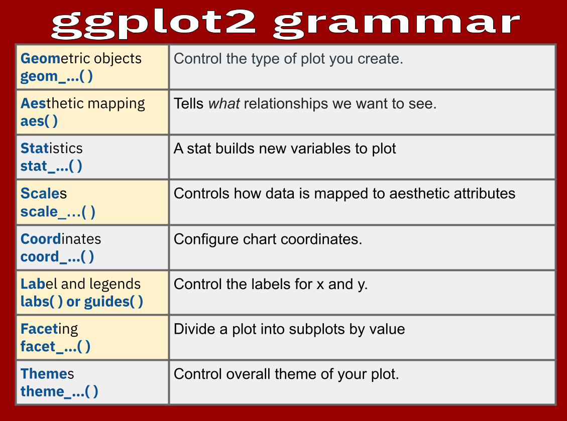
Exploration with Data Visualization using ggplot2
ggplot2 is designed to work iteratively. You start with a layer that shows the raw data, then add layers of annotations and statistical summaries. ggplot2 is a part of the tidyverse, so we do not need to load it again.
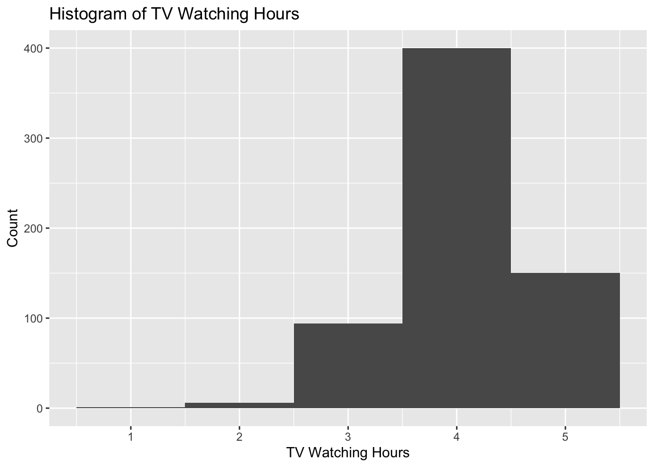
# Add dataggplot(data_to_explore, aes(x = tv)) +geom_histogram(bins =5) +#specifies that the variable gets sorted into 5 bins# Add the labelslabs(title ="Histogram of TV Watching Hours",caption ="Approximately how many students watch 4+ hours of TV per day?",x ="TV Watching Hours",y ="Count")
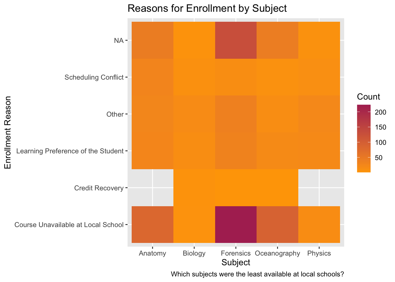
Two categorical variables: Heatmap
Create a basic visualization that examines the relationship between two categorical variables using a heatmap via geom_tile().
For this visualization, we will be guided by the following research question:
❓ What are the reasons for enrollment in various courses?
We can make a heatmap (via geom_tile()) to visualize the relationship between the course subject and reasons for enrollment.
👉 Your Turn⤵
Data: data_to_explore
First, use the count() function for the categorical variables subject & enrollment, then
ggplot()
aes():
subject mapped to x position
enrollment_reason mapped to y position
Geom: geom_tile()
Title: “Reasons for Enrollment by Subject”
Caption: “Which subjects were the least available at local schools?”
We’ve added extra code as scale_fill_gradient() and labs() to help show a heatmap’s effectiveness. Play around with it if you’d like!
data_to_explore %>%count(subject, enrollment_reason) %>%ggplot(aes(x = subject, y = enrollment_reason, fill = n)) +geom_tile() +scale_fill_gradient(low ="orange", high ="maroon") +#Try changing one color to "red"!labs(title ="Reasons for Enrollment by Subject",caption ="Which subjects were the least available at local schools?",x ="Subject",y ="Enrollment Reason",fill ="Count")
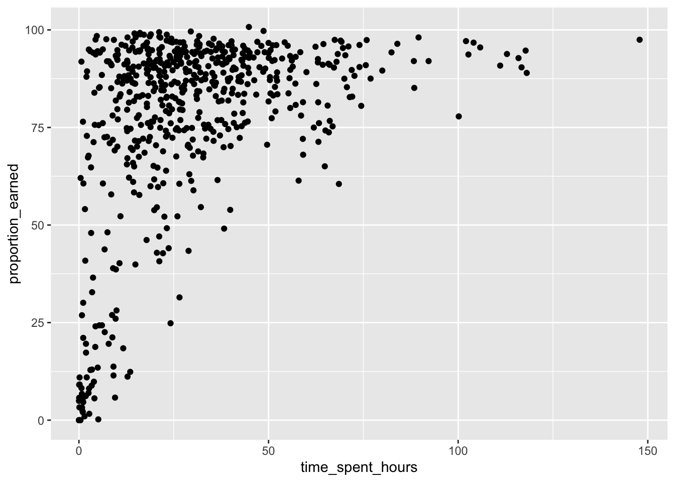
Two continuous variables: Scatter plot
Create a basic visualization that examines the relationship between two continuous variables using a scatter plot via geom_point().
For this visualization, we will be guided by the following research question:
❓ Can we predict the grade on a course from the time spent in the course LMS?
👉 Your turn⤵
Take another look at your data:
#look at the data frame#(add code below)head(data_to_explore)
#(add code below)#layer 1: add data and aesthetics mapping ggplot(data_to_explore,aes(x = time_spent_hours, y = proportion_earned)) +#layer 2: + geom function typegeom_point()
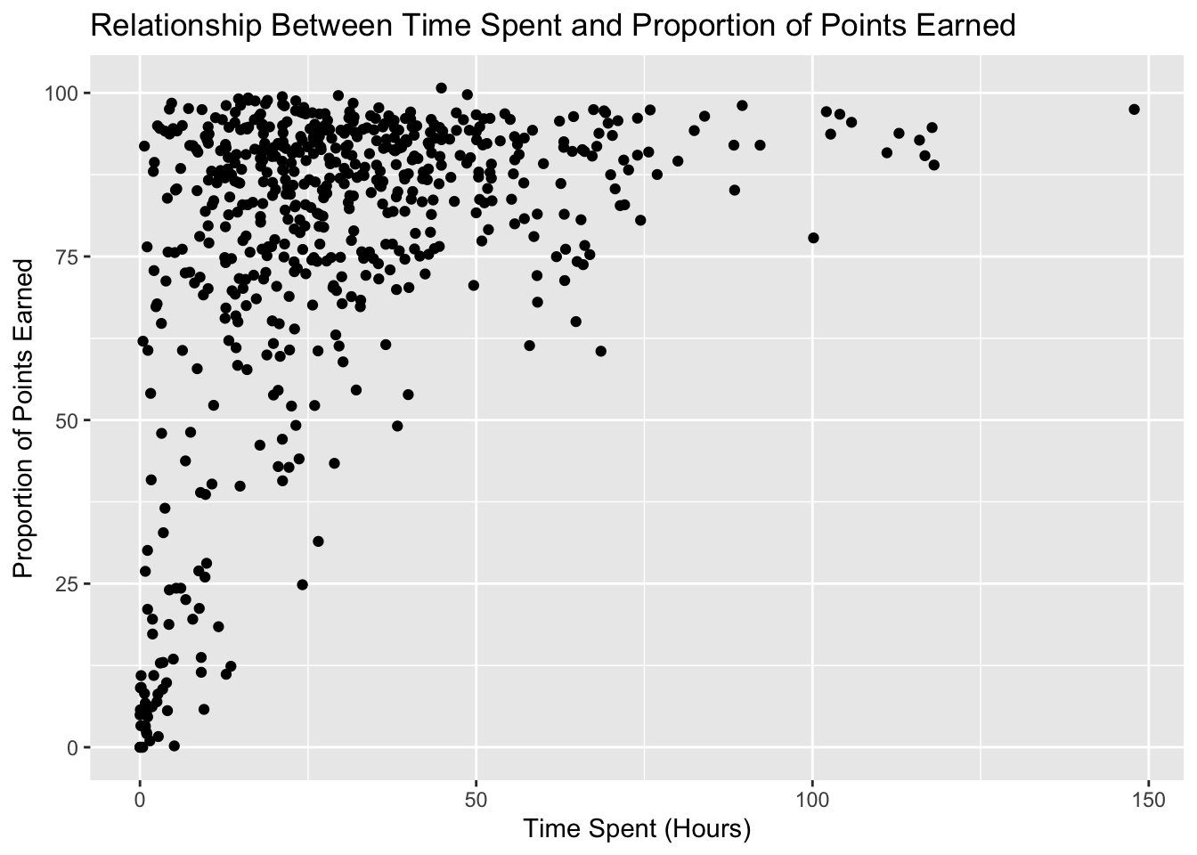
Level b. Add another layer with labels
👉 Your Turn⤵
Title: “How Time Spent on Course LMS is Related to Points Earned in the course”
x label: “Time Spent (Hours)”
y label: “Proportion of Points Earned”
#(add code below)ggplot(data_to_explore, aes(x = time_spent_hours, y = proportion_earned)) +geom_point() +labs(title ="Relationship Between Time Spent and Proportion of Points Earned",x ="Time Spent (Hours)",y ="Proportion of Points Earned")
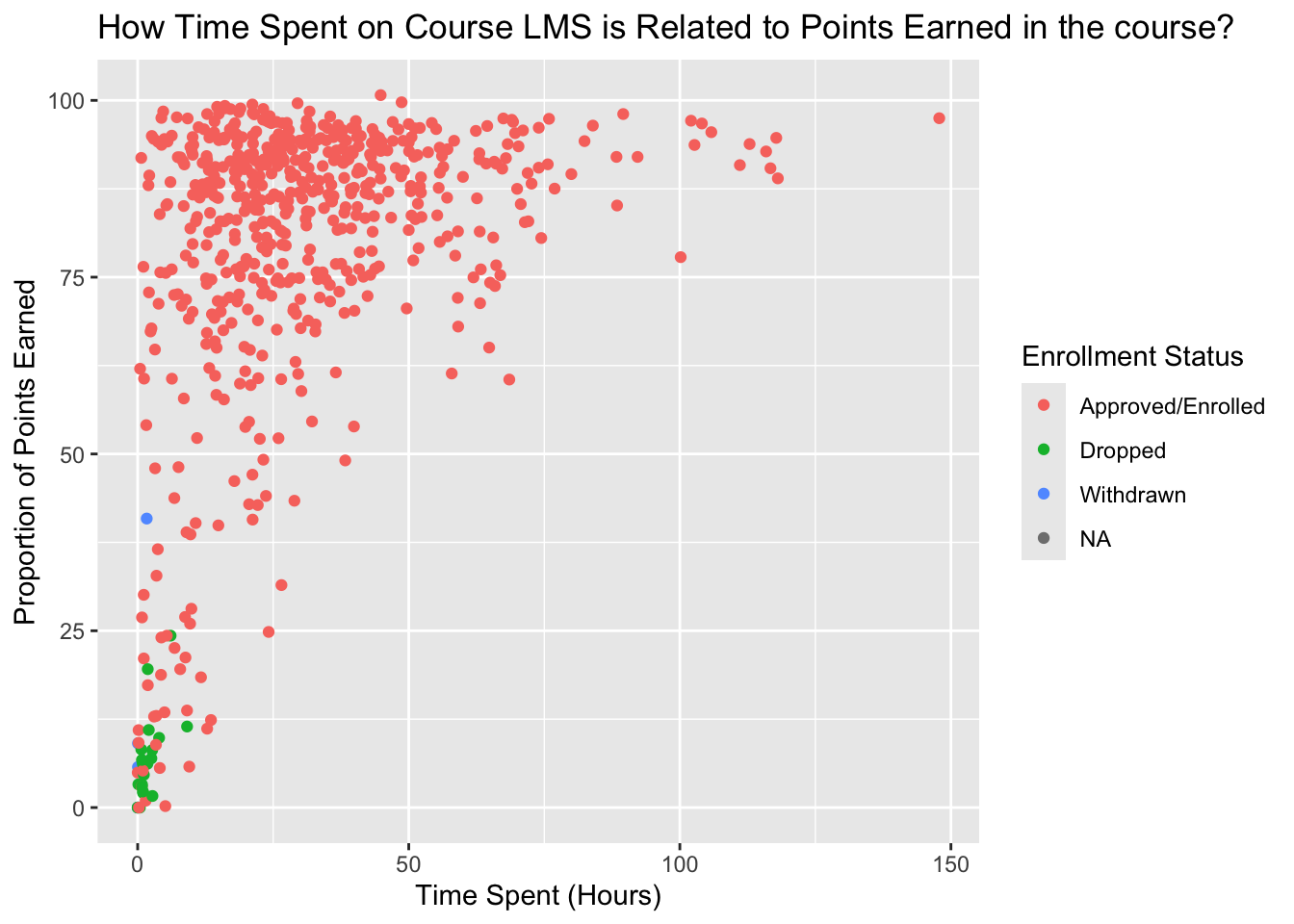
Level c. Add scale with a different color.
❓ Can we notice anything about enrollment status?
We’ll add scale by telling the aes() function to make the colors of the points correspond to the enrollment_status variable.
👉 Your Turn⤵
Create a scatter plot with color based on enrollment_status.
#(add code below)ggplot(data_to_explore, aes(x = time_spent_hours, y = proportion_earned, color = enrollment_status)) +geom_point() +labs(title ="How Time Spent on Course LMS is Related to Points Earned in the course?",x ="Time Spent (Hours)",y ="Proportion of Points Earned",color ="Enrollment Status")
Level d. Divide up graphs using facet to visualize by subject.
The facet_wrap() function allows you to generate multiple visualizations side-by-side for easier comparison. We’ll use subject as the variable.
👉 Your Turn⤵
Create a scatter plot with facets for each subject using facet_wrap().
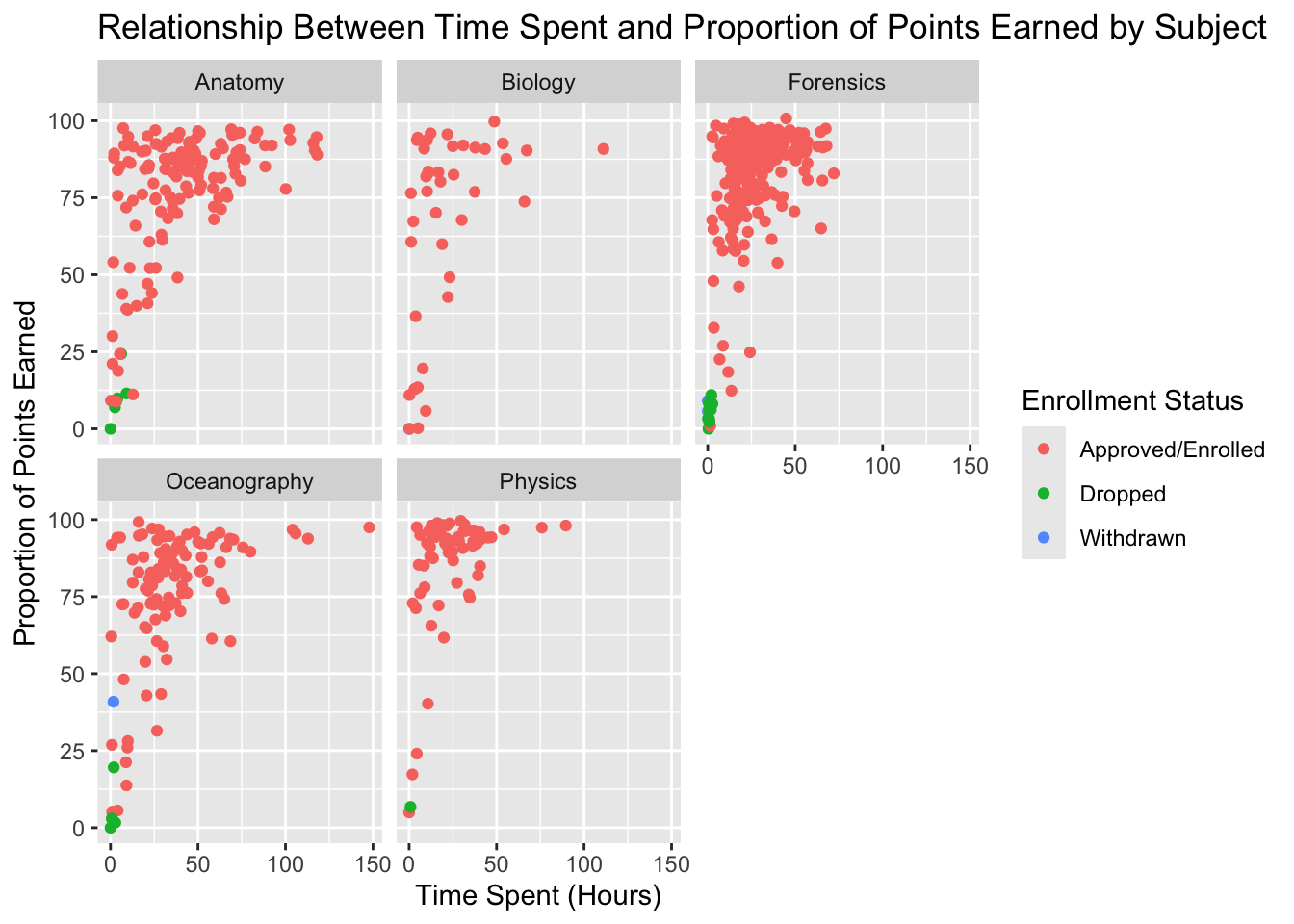
#(add code below)ggplot(data_to_explore, aes(x = time_spent_hours, y = proportion_earned, color = enrollment_status)) +geom_point() +facet_wrap(~subject) +labs(title ="Relationship Between Time Spent and Proportion of Points Earned by Subject",x ="Time Spent (Hours)",y ="Proportion of Points Earned",color ="Enrollment Status")
Level e. Remove NAs from plot
Start with data_to_explore.
Pipe in an argument to drop_na() from:
time_spent_hours
proportion_earned
enrollment_status
Use your previous ggplot() code from above. Remember that you already piped in data_to_explore, so you can remove it from the first argument after ggplot().
#(add code here)data_to_explore %>%drop_na(time_spent_hours, proportion_earned, enrollment_status, subject) %>%ggplot(aes(x = time_spent_hours, y = proportion_earned, color = enrollment_status)) +geom_point() +labs(title ="Relationship Between Time Spent and Proportion of Points Earned by Subject",x ="Time Spent (Hours)",y ="Proportion of Points Earned",color ="Enrollment Status") +facet_wrap(~subject)
As Alex explores the data through visualizations and summary statistics, she begins to see trends that could indicate which students are at risk. Her observations guide her to consider changes in her teaching approach or additional support for certain students.
🛑 Stop here! Congratulations, you finished the second part of the case study.
4. MODEL (Module 3)
As highlighted in.Chapter 3 of Data Science in Education Using R, the Model step of the data science process entails “using statistical models, from simple to complex, to understand trends and patterns in the data.”
The authors note that while descriptive statistics and data visualization during the Explore step can help us to identify patterns and relationships in our data, statistical models can be used to help us determine if relationships, patterns and trends are actually meaningful.
Simple Correlation
As highlighted in @macfadyen2010, scatter plots are a useful initial approach for identifying potential correlational trends between variables under investigation, but to further interrogate the significance of selected variables as indicators of student achievement, a simple correlation analysis of each variable with student final grade can be conducted.
There are two efficient ways to create correlation matrices, one that is best for internal use, and one that is best for inclusion in a manuscript.
correlate()
The corrr package provides a way to create a correlation matrix in a tidyverse-friendly way. Like for the skimr package, it can take as little as a line of code to create a correlation matrix. If unfamiliar, a correlation matrix is a table that presents how all of the variables are related to all of the other variables.
👉 Your Turn⤵
First, load the corrr package using the correct function. You may need to install.packages() in the console if this is your first time using loading the package.
# load in corrr library#(add code below)library(corrr)
Attaching package: 'corrr'
The following object is masked from 'package:skimr':

    focus
Look and see if there is a simple correlation between time spent in hours and the proportion of points earned:
# A tibble: 2 × 3
  term              proportion_earned time_spent_hours
  <chr>                         <dbl>            <dbl>
1 proportion_earned            NA                0.438
2 time_spent_hours              0.438           NA
fashion()
For printing purposes, the fashion() function can be added for converting a correlation into a cleanly formatted matrix, with leading zeros removed, spaces for signs, and the diagonal (or any NA) left blank.
               term proportion_earned time_spent_hours
1 proportion_earned
2  time_spent_hours               .44
👉 Your Turn⤵
❓ What could we write up for a manuscript in APA format or another format? Offer a short summary below:
In the study, Pearson’s correlation coefficient was calculated to assess the relationship between the proportion of course materials earned and the time spent in hours. The analysis revealed a moderate positive correlation of .44 between these variables, suggesting that as the time students spent on course materials increased, so did their proportion of earned materials (pairwise complete observations were used to handle missing data).
❓ What other variables would you like to check out?
[YOUR RESPONSE HERE]
Take some of those variables and explore them using correlate():
#(add code below)
APA Formatting
While corrr is a nice package to quickly create a correlation matrix, you may wish to create one that is ready to be added directly to a dissertation or journal article. apaTables is great for creating more formal forms of output that can be added directly to an APA-formatted manuscript. It also has functionality for regression and other types of model output.
However, apaTables is not as friendly to tidyverse functions. First, we need to select only the variables we wish to correlate. Then, we can use that subset of the variables as the argument to the apa.cor.table() function.
👉 Your Turn⤵
Run the following code to create a subset of the larger data_to_explore data frame with the variables you wish to correlate, then create a correlation table using apa.cor.table().
Load apaTables library.
Save your selected variables for comparison to a new object data_to_explore_subset.
Means, standard deviations, and correlations with confidence intervals


  Variable             M     SD    1           2
  1. time_spent_hours  30.48 22.72

  2. proportion_earned 76.23 25.20 .44**
                                   [.37, .50]

  3. int               4.30  0.60  .08         .14**
                                   [-.01, .16] [.06, .22]


Note. M and SD are used to represent mean and standard deviation, respectively.
Values in square brackets indicate the 95% confidence interval.
The confidence interval is a plausible range of population correlations
that could have caused the sample correlation (Cumming, 2014).
 * indicates p < .05. ** indicates p < .01.
This may look nice, but how do we add this into a dissertation or article that you might be interested in publishing?
Read the documentation for apa.cor.table() by running ?apa.cor.table() in the console. Look through the documentation and examples to understand how to output a file with the formatted correlation table, and then run the code to do that with your subset data_to_explore_subset.
Means, standard deviations, and correlations with confidence intervals


  Variable             M     SD    1           2
  1. time_spent_hours  30.48 22.72

  2. proportion_earned 76.23 25.20 .44**
                                   [.37, .50]

  3. int               4.30  0.60  .08         .14**
                                   [-.01, .16] [.06, .22]


Note. M and SD are used to represent mean and standard deviation, respectively.
Values in square brackets indicate the 95% confidence interval.
The confidence interval is a plausible range of population correlations
that could have caused the sample correlation (Cumming, 2014).
 * indicates p < .05. ** indicates p < .01.
You should now see a new Word document in your project folder called survey-cor-table.doc. Click on that and you’ll be prompted to download from your browser.
Linear Regression
In brief, a linear regression model involves estimating the relationships between one or more independent variables with one dependent variable. Mathematically, it can be written like the following.
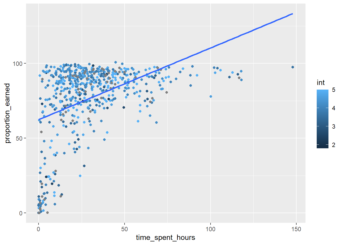
Use lm() to estimate a model in which proportion_earned is the dependent variable. It is predicted by one independent variable, time_spent_hours, with an interaction term int (interest in science).
#(add code here)lm(proportion_earned ~ time_spent_hours +int, data = data_to_explore)
Call:
lm(formula = proportion_earned ~ time_spent_hours + int, data = data_to_explore)

Coefficients:
     (Intercept)  time_spent_hours               int
         44.9657            0.4255            4.6283
We can see that the intercept is now estimated at 44, which tells us that when students’ time spent and interest are equal to zero, they are likely fail the course (unsurprisingly). Note that that estimate for interest in science is 4.6, so for every one-unit increase in int, we should expect about a 5 percentage point increase in their grade.
We can save the output of the function to an object. Let’s call it m1 for “Model 1.” We can then use the summary() function built into R to view a much more feature-rich summary of the estimated model.
# save the modelm1 <-lm(proportion_earned ~ time_spent_hours + int, data = data_to_explore)
👉 Your Turn⤵
Run a summary for the model you just created, called m1.
#run the summarysummary(m1)
Call:
lm(formula = proportion_earned ~ time_spent_hours + int, data = data_to_explore)

Residuals:
    Min      1Q  Median      3Q     Max
-66.705  -7.836   5.049  14.695  35.766

Coefficients:
                 Estimate Std. Error t value Pr(>|t|)
(Intercept)       44.9657     6.6488   6.763 3.54e-11 ***
time_spent_hours   0.4255     0.0410  10.378  < 2e-16 ***
int                4.6283     1.5364   3.012  0.00271 **
---
Signif. codes:  0 '***' 0.001 '**' 0.01 '*' 0.05 '.' 0.1 ' ' 1

Residual standard error: 21.42 on 536 degrees of freedom
  (404 observations deleted due to missingness)
Multiple R-squared:  0.1859,    Adjusted R-squared:  0.1828
F-statistic: 61.18 on 2 and 536 DF,  p-value: < 2.2e-16
Let’s save this as a nice APA table for possible publication.
# use the {apaTables} package to create a nice regression table that could be used for later publication.apa.reg.table(m1, filename ="lm-table.doc")
Regression results using proportion_earned as the criterion


        Predictor       b       b_95%_CI beta  beta_95%_CI sr2  sr2_95%_CI
      (Intercept) 44.97** [31.90, 58.03]
 time_spent_hours  0.43**   [0.34, 0.51] 0.41 [0.33, 0.48] .16  [.11, .22]
              int  4.63**   [1.61, 7.65] 0.12 [0.04, 0.19] .01 [-.00, .03]


     r             Fit

 .41**
 .15**
           R2 = .186**
       95% CI[.13,.24]


Note. A significant b-weight indicates the beta-weight and semi-partial correlation are also significant.
b represents unstandardized regression weights. beta indicates the standardized regression weights.
sr2 represents the semi-partial correlation squared. r represents the zero-order correlation.
Square brackets are used to enclose the lower and upper limits of a confidence interval.
* indicates p < .05. ** indicates p < .01.
By creating simple models, Alex hopes to predict student outcomes more accurately. She is interested in how variables like time spent on tasks correlate with student grades and uses this information to adjust her instructional strategies.
Summarize predictors
The summarize() function from the dplyr package creates summary statistics such as the mean, standard deviation, or the minimum or maximum of a value. At its core, think of summarize() as a function that returns a single statistics summarizing a single column.
👉 Your Turn⤵
In the space below find the mean int of students using summarize(), removing any NAs.
The mean value for interest is quite high. If we multiply the estimated relationship between interest and proportion of points earned—0.046—by this, the mean interest across all of the students—we can determine that students’ estimated final grade was 0.046 X 4.3, or 0.197.
👉 Your Turn⤵
Do the same for time_spent_hours by finding the mean and removing any NAs using summarize().
For hours spent, the average students’ estimated final grade was 0.0042 X 30.48, or 0.128.
If we add both 0.197 and 0.128 to the intercept, 0.449, that equals 0.774, or about 77%. In other words, a student with average interest in science who spent an average amount of time in the course earned a pretty average grade.
Checking Assumptions
Great! Now that you have defined your linear model m1 in R, which predicts proportion_earned based on time_spent_hours and the interaction term int.
Let’s go through how to check the assumptions of this linear model using the various diagnostic plots and tests.
We’ll need to check:
Linearity and Interaction Effects
Residuals Analysis
Normality of Residuals
Multicollinearity
Linearity and Interaction Effect
Since our model includes an interaction term (int), it’s good to first check if the interaction is meaningful and whether the linearity assumption holds for the predictors in relation to the dependent variable.
Warning: Removed 345 rows containing non-finite outside the scale range
(`stat_smooth()`).
Warning: The following aesthetics were dropped during statistical transformation:
colour.
ℹ This can happen when ggplot fails to infer the correct grouping structure in
  the data.
ℹ Did you forget to specify a `group` aesthetic or to convert a numerical
  variable into a factor?
Warning: Removed 345 rows containing missing values or values outside the scale range
(`geom_point()`).
This plot helps visualize if the interaction term significantly affects the relationship between your predictors and the dependent variable.
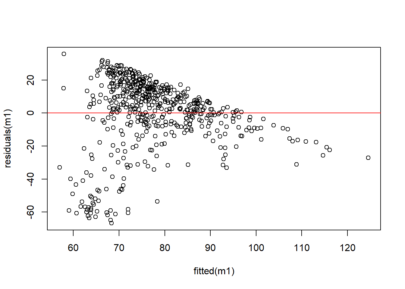
Residuals Analysis
Next, we’ll plot the residuals against the fitted values to check for independence, homoscedasticity, and any unusual patterns.
plot(residuals(m1) ~fitted(m1))abline(h =0, col ="red")
Look for a random dispersion of points. Any pattern or funnel shape indicates issues with homoscedasticity or linearity.
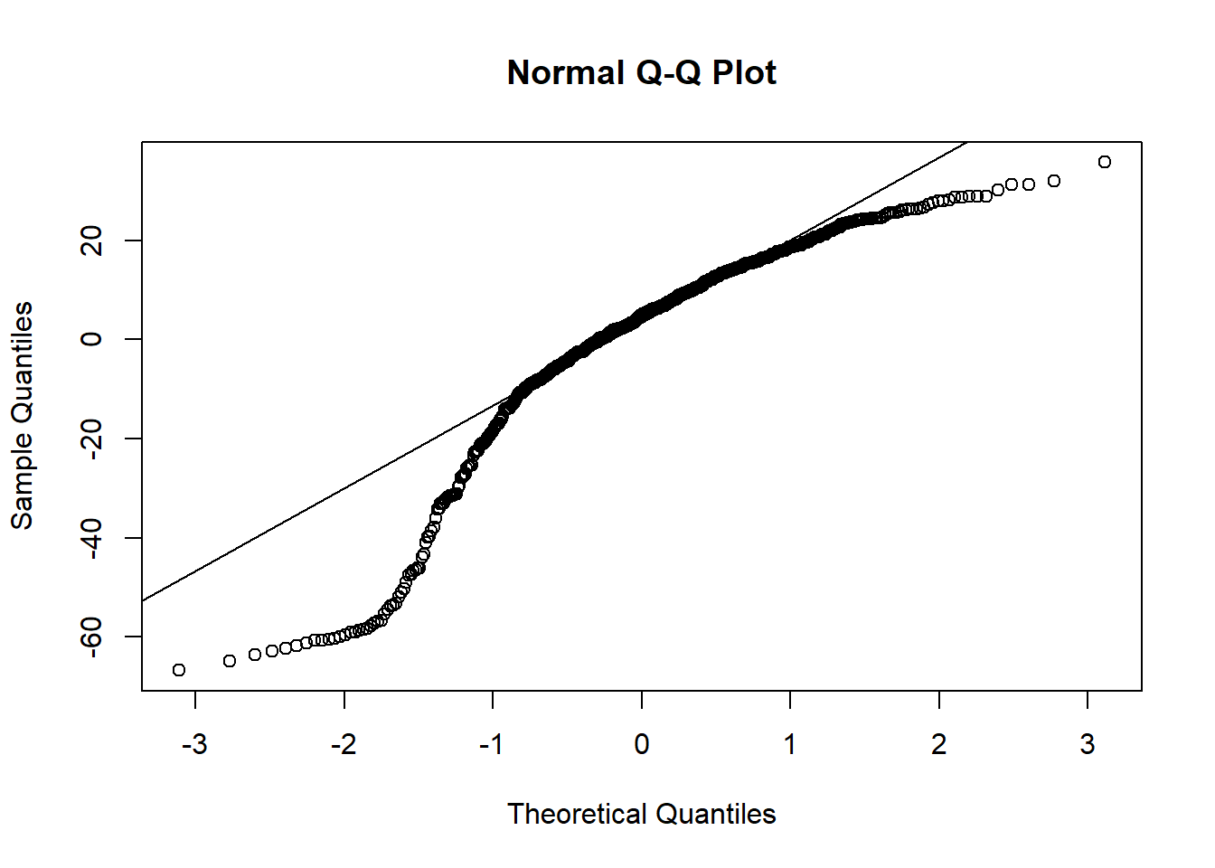
Normality of Residuals
A deviation from the straight line in the Normal Q-Q plot indicates deviations from normality.
qqnorm(residuals(m1))qqline(residuals(m1))
The Shapiro-Wilk test is another way to test normality.
shapiro.test(residuals(m1))
    Shapiro-Wilk normality test

data:  residuals(m1)
W = 0.88967, p-value < 2.2e-16
W statistic: The test statistic W is 0.88967. This value indicates the extent to which the data are normally distributed. W values close to 1 suggest that the data closely follow a normal distribution. In this case, a W value of 0.88967 suggests some deviation from normality.
p-value: The p-value is less than 2.2e-16 (a very small number close to zero). In statistical testing, a p-value less than the chosen significance level (typically 0.05) leads to the rejection of the null hypothesis.
Multicollinearity
We can use vif() from the car package to identify multicolinearity. You try it!
👉 Your Turn⤵
Load the package car.
Use the vif() function for your model m1.
#(add code below)library(car)
Warning: package 'car' was built under R version 4.5.2
Loading required package: carData
Warning: package 'carData' was built under R version 4.5.2
Attaching package: 'car'
The following object is masked from 'package:dplyr':

    recode
The following object is masked from 'package:purrr':

    some
vif(m1)
time_spent_hours              int
        1.006076         1.006076
Interpretation of VIF Scores
VIF Value
Interpretation
= 1
No correlation among the predictor and all other predictors
< 5
Generally indicates a moderate level of multicollinearity
>= 5 to 10
May indicate a problematic amount of multicollinearity, depending on the context and sources
>10
Signifies high multicollinearity that can severely distort the least squares estimates
Both of the VIF scores are slightly above 1, which suggests that there is almost no multicollinearity among these predictors. This is a good sign, indicating that each predictor provides unique and independent information to the model, not unduly influenced by the other variables.
Our model was violated and does not follow a normality. However, we are going to practice other functions as if it passed all assumptions. Assumption testing is just for you to know how to do in the future. You will need to correct issues like normality by exploring data transformations, adding polynomial or interaction terms to the model, or using a different type of regression model that does not assume normality of residuals.
🛑 Stop here! Congratulations, you finished the third part of the case study.
5. COMMUNICATE (Module 4)
For your final 👉 Your Turn, your goal is to distill our analysis into a Quarto “data product” designed to illustrate key findings. Feel free to use the template in the lab 4 folder.
The final step in the workflow/process is sharing the results of your analysis with wider audience. Krumm et al. @krumm2018 have outlined the following 3-step process for communicating with education stakeholders findings from an analysis:
Select. Communicating what one has learned involves selecting among those analyses that are most important and most useful to an intended audience, as well as selecting a form for displaying that information, such as a graph or table in static or interactive form, i.e. a “data product.”
Polish. After creating initial versions of data products, research teams often spend time refining or polishing them, by adding or editing titles, labels, and notations and by working with colors and shapes to highlight key points.
Narrate. Writing a narrative to accompany the data products involves, at a minimum, pairing a data product with its related research question, describing how best to interpret the data product, and explaining the ways in which the data product helps answer the research question and might be used to inform new analyses or a “change idea” for improving student learning.
👉 Your Turn⤵
Create a data story with our current data set, or your own. Make sure to use the LA workflow as your guide to include:
Develop a research question
Add ggplot visualizations
Offer a model (with visualizations)
Communicate by writing up a short write up for intended stakeholders. Remember to write it in terms the stakeholders understand.
[ENTER YOUR RESPONSE HERE]
Finally, Alex prepares to communicate her findings. She creates a simple web page using Markdown to share her insights with colleagues. This acts as a practical example of how data can inform teaching practices.
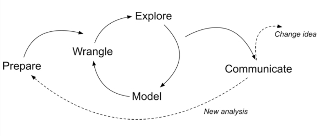
 Alex begins by understanding the importance of data analysis in identifying students who might need extra support. The cited foundational study motivates her to explore similar analyses to develop her own early warning system.