Model

Foundations Python Module 3: Code-A-long

Welcome to Foundations code along for Module 3

Modeling for educational researchers builds on insights from Exploratory Data Analysis (EDA) to develop predictive or explanatory models that guide decision-making and enhance learning outcomes.

This involves selecting appropriate models, preparing and transforming data, training and validating the models, and interpreting results. Effective modeling helps uncover key factors influencing educational success, allowing for targeted interventions and informed policy decisions.

Modeling for educational researchers is a crucial step following Exploratory Data Analysis (EDA) in the learning analytics workflow. This stage involves developing predictive or explanatory models that guide decision-making and enhance educational outcomes. The process begins with clearly defining research questions or hypotheses based on insights from EDA. Researchers then select appropriate models, prepare and transform data through cleaning and feature engineering, and train and validate the models by splitting data into training and validation sets. Analyzing model outputs, such as feature importances, helps uncover key factors influencing educational success.

Module Objectives

By the end of this module:

• Introduction to Modeling:
  • Learners will understand the importance of modeling in the learning analytics workflow and how it helps quantify insights from data.

• Creating and Interpreting Correlations:
  • Learners will create and interpret correlation matrices using the {corrr} package and create APA-formatted correlation tables using the {apaTables} package.

• Applying Various Modeling Techniques:
  • Learners will fit and understand linear regression models to prepare for the case study.

In this module, we will focus on the practical aspects of modeling within the learning analytics workflow. By the end of this module, students will understand the importance of modeling and how it fits into the overall data analysis process. We will specifically cover the steps involved in creating and interpreting correlation matrices, fitting linear regression models, and validating model assumptions using R.

We’ll begin by learning how to create and interpret correlation matrices using the {corrr} package. This will help us identify and understand relationships between different variables in our data. We’ll also explore how to create APA-formatted correlation tables using the {apaTables} package, which are useful for formal reports and publications.

Next, we’ll apply various modeling techniques, starting with fitting linear regression models to predict academic achievement. We will also discuss the importance of validating model assumptions to ensure our models are robust and reliable. Additionally, we’ll use the summarize() function from the {dplyr} package to calculate summary statistics for our predictors, helping us to better understand our data and inform our modeling process. By the end of this module, students will have practical experience with these modeling techniques, enabling them to perform more advanced data analysis in their research.

Steps in the Modeling Process

Speaker notes

Th modeling phase is important for transforming the insights gained from Exploratory Data Analysis (EDA) into actionable predictions and explanations using statistical models.

Defining Objectives and Hypotheses:

The first step in modeling is to clearly define the objectives and hypotheses based on the insights gathered from EDA. This sets the direction for the modeling process and ensures that we are addressing the right questions.

Selecting Appropriate Models: Once we have our objectives, the next step is to select the appropriate models. This involves choosing the statistical or machine learning techniques that best fit our data and research questions. We will look at various models, such as linear regression, decision trees, and more complex algorithms.

Data Preparation and Feature Engineering:

Preparing the data is crucial for building effective models. This includes cleaning the data, handling missing values, and performing feature engineering to create new variables that better represent the underlying patterns in the data. We will use R to demonstrate these processes. Model Training and Validation:

After preparing the data, we move on to training our models. This involves fitting the models to our training data and using validation techniques to assess their performance. We will discuss the importance of splitting data into training and validation sets and using cross-validation to ensure robustness.

Interpreting Model Results:

Once the models are trained, we need to interpret the results. This step involves understanding the model outputs, such as coefficients in a regression model or feature importances in a tree-based model. We will learn how to extract meaningful insights from these results.

Assessing Model Performance:

Assessing model performance is critical to ensure that our models are accurate and reliable. We will use various metrics, such as accuracy, precision, recall, and RMSE, to evaluate the performance of our models and compare different models.

Refining and Tuning Models:

The final step in the modeling process is refining and tuning our models. This involves adjusting hyperparameters, experimenting with different algorithms, and performing feature selection to improve model performance. We will explore techniques for optimizing our models to achieve the best possible results.

Dummy Data

• Create dummy data
• Introduce NaN

# Creating demo data
import pandas as pd
import numpy as np

# Seed for reproducibility
np.random.seed(42)

# Create demo data
demo_data = pd.DataFrame({
    'completion_percentage': np.random.uniform(50, 100, 100),  # Completion between 50% and 100%
    'hours_online': np.random.uniform(1, 50, 100),             # Hours online between 1 and 50
    'boredom_score': np.random.uniform(1, 5, 100)              # Boredom score between 1 and 5
})

• Purpose: The .loc function in Pandas is a powerful tool for accessing and modifying data in a DataFrame.

• Functionality: It allows for selection by label and the assignment of new values to those selected locations.

# Introduce some NaN values
demo_data.loc[np.random.choice(demo_data.index, size=10, replace=False), 'completion_percentage'] = np.nan
demo_data.loc[np.random.choice(demo_data.index, size=10, replace=False), 'hours_online'] = np.nan
demo_data.loc[np.random.choice(demo_data.index, size=10, replace=False), 'boredom_score'] = np.nan

Creating dummy data goal is to create a realistic set of data that we can work with to understand various functions and methods in data analysis.

First, we set a seed for reproducibility using np.random.seed(42). This ensures that every time we run this code, we will get the same set of random numbers. Reproducibility is essential in data analysis because it allows us to verify results and ensure that our findings are consistent.

Next, we generate our demo data using the pd.DataFrame() function from the Pandas library. We create a DataFrame with three columns:

completion_percentage: This column contains random values between 50% and 100%, representing the percentage of course completion by students. hours_online: This column includes random values between 1 and 50, indicating the number of hours students spend online. boredom_score: This column has random values between 1 and 5, representing a self-reported score of how bored students feel during their online sessions. Each of these columns is populated with 100 random values, which will provide a robust dataset for our subsequent analysis and modeling exercises.

By setting up our demo data in this way, we can simulate a realistic scenario where we have to handle various types of data and potential issues, such as missing values or data imputation, which we will address in later sections.

Introduce NaN .loc function allows us to select data by label, and we can also assign new values to those selected locations. This is particularly helpful when we want to introduce missing values or simulate specific data conditions.

In our example, we are introducing NaN values into specific columns to simulate missing data. We use the np.random.choice function to randomly select 10 indices from our DataFrame, ensuring no index is selected more than once with replace=False.

We then use .loc to assign NaN values to the selected indices in the completion_percentage, hours_online, and boredom_score columns.

Correlation

• Corr()
• Discussion

The corr() method (in Pandas) calculates the relationship between each column in your data set.

# Select specific variables for analysis
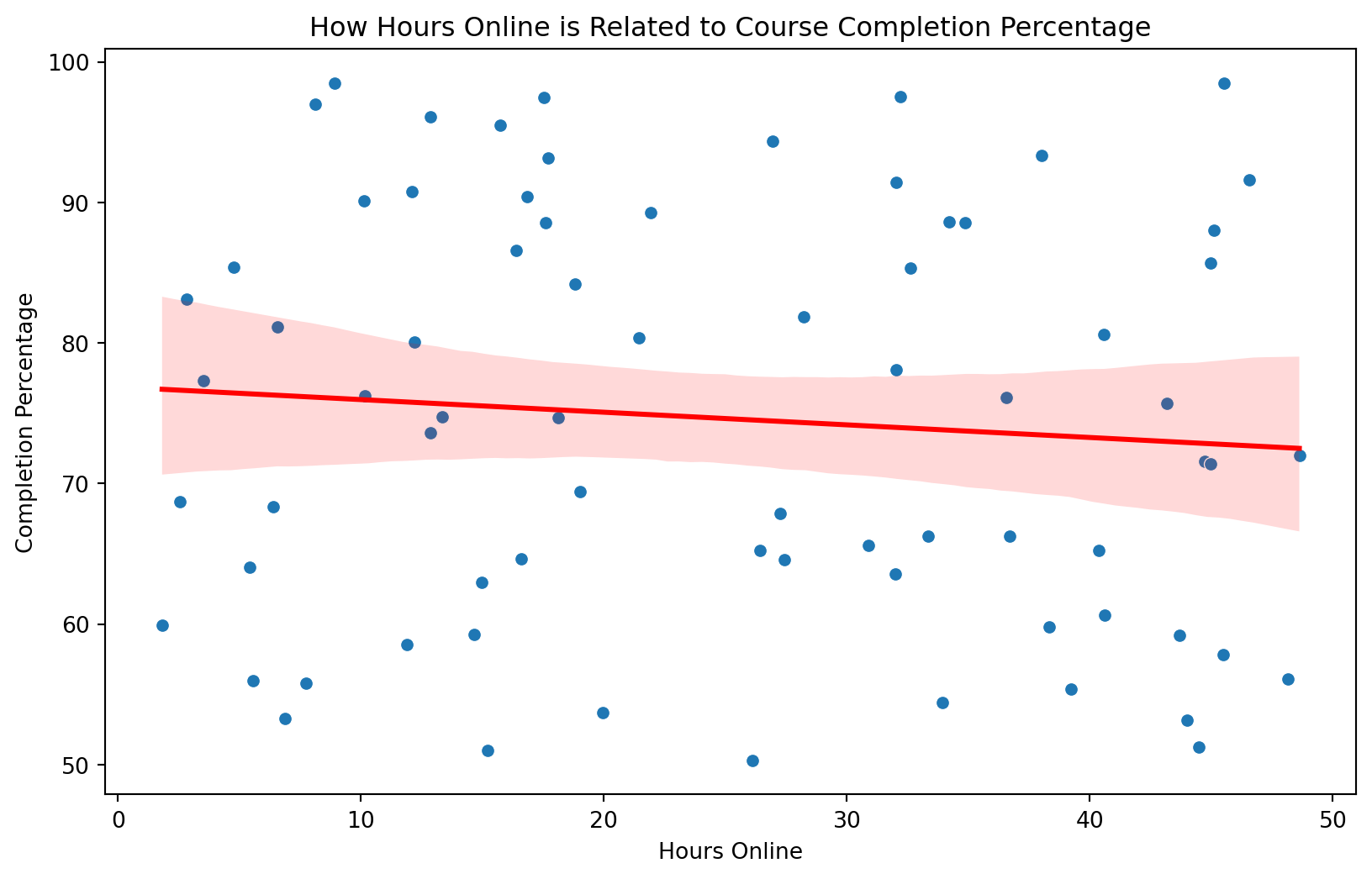
selected_data = demo_data[['completion_percentage', 'hours_online']]

# Calculate the correlation matrix
correlation_matrix = selected_data.corr()

# Print the correlation matrix
print(correlation_matrix)

                       completion_percentage  hours_online
completion_percentage               1.000000     -0.094677
hours_online                       -0.094677      1.000000

What is the interpretation of -.095 correlation?

Correlation

Discussion

The correlation matrix provides the pairwise correlations between the selected variables, allowing us to understand the relationships between them. Specifically, the correlation coefficient between completion_percentage and hours_online is -0.094677. This value is close to 0, indicating a very weak negative correlation.

A negative correlation suggests that as one variable increases, the other tends to decrease. However, in this case, the relationship is very weak. The diagonal values in the matrix are always 1.000000, representing the correlation of each variable with itself.

Interpreting this, the correlation coefficient of -0.094677 between completion_percentage and hours_online implies a very weak negative relationship between these two variables. Practically, this means that there is almost no linear relationship between the hours spent online and the completion percentage. The negative sign indicates a slight tendency for the completion percentage to decrease as hours online increase, but this trend is not strong enough to be of significant concern.

Linear Regression

• package 👉 Your Turn ⤵
• Answer
• Regression
• Code and output

Linear regression is implemented using the statsmodels library

Add the statsmodels.api packages as sm

👉 Your Turn ⤵ -> Answer

#import stats model
import statsmodels.api as sm

Instructions:

1. Clean the data

2. Create a linear regression model with hours_online as the independent variable and completion_percentage as the dependent variable.

3. Fit the model and inspect the summary.

4. Visualize the model with a scatter plot and regression line

# Step 1: Drop rows with missing values
data_cleaned = selected_data.dropna()

# Step 2: Define independent and dependent variables
X = data_cleaned[['hours_online']]  # Independent variable
y = data_cleaned['completion_percentage']  # Dependent variable

# Step 3: Add a constant to the model (for the intercept)
X = sm.add_constant(X)

# Step 4: Fit the model
model = sm.OLS(y, X).fit()

# Step 5: Output the summary of the model
print(model.summary())

                              OLS Regression Results                             
=================================================================================
Dep. Variable:     completion_percentage   R-squared:                       0.009
Model:                               OLS   Adj. R-squared:                 -0.003
Method:                    Least Squares   F-statistic:                    0.7236
Date:                   Mon, 22 Jul 2024   Prob (F-statistic):              0.398
Time:                           21:01:38   Log-Likelihood:                -335.86
No. Observations:                     82   AIC:                             675.7
Df Residuals:                         80   BIC:                             680.5
Df Model:                              1                                         
Covariance Type:               nonrobust                                         
================================================================================
                   coef    std err          t      P>|t|      [0.025      0.975]
--------------------------------------------------------------------------------
const           76.2415      3.254     23.433      0.000      69.767      82.716
hours_online    -0.0957      0.112     -0.851      0.398      -0.320       0.128
==============================================================================
Omnibus:                       30.477   Durbin-Watson:                   2.093
Prob(Omnibus):                  0.000   Jarque-Bera (JB):                5.312
Skew:                           0.038   Prob(JB):                       0.0702
Kurtosis:                       1.755   Cond. No.                         57.9
==============================================================================

Notes:
[1] Standard Errors assume that the covariance matrix of the errors is correctly specified.

Defining Variables:

We define the independent variable (X) as hours_online and the dependent variable (y) as completion_percentage. We add a constant to the model to account for the intercept. Fitting the Model:

Using the statsmodels library, we fit an Ordinary Least Squares (OLS) regression model. statsmodels is a powerful library specifically designed for statistical modeling in Python. The summary() function provides detailed statistics about the model, including coefficients, R-squared value, and p-values.

Multiple regression

• 👉 Your Turn ⤵
• Answer
• Bonus - Visualize
• Bonus - ANSWER

Instructions:

1. Clean the data using the dropna() function

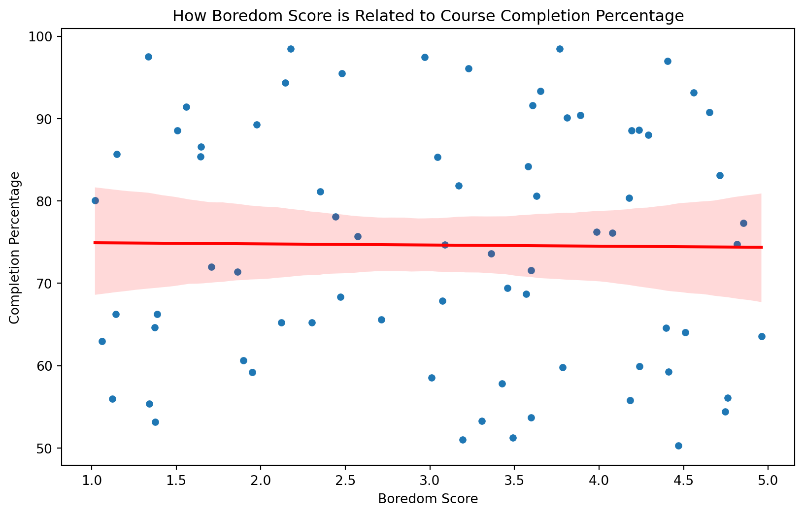
2. Create a linear regression model with hours_online and boredom_score as the independent variable and completion_percentage as the dependent variable.

3. Fit the model and inspect the summary.

#install libraries
import seaborn as sns #seaborn
import matplotlib.pyplot as plt #matplot

# Step 1: Drop rows with missing values in any of the selected columns
cleaned_data = demo_data.dropna()

# Step 1a: Verify that there are no missing values in cleaned_data
print(cleaned_data.isna().sum())

# Steps 2, add independent and dependent variables to X and y
X = cleaned_data[['hours_online', 'boredom_score']]  # independent variables
y = cleaned_data['completion_percentage']  # dependent variable

# Adding a constant to the model (for the intercept)
X = sm.add_constant(X)

# Steps 4 and 5 to Fit the model
model = sm.OLS(y, X, missing='drop').fit()

# Output the summary of the model
print(model.summary())

completion_percentage    0
hours_online             0
boredom_score            0
dtype: int64
                              OLS Regression Results                             
=================================================================================
Dep. Variable:     completion_percentage   R-squared:                       0.009
Model:                               OLS   Adj. R-squared:                 -0.019
Method:                    Least Squares   F-statistic:                    0.3072
Date:                   Mon, 22 Jul 2024   Prob (F-statistic):              0.736
Time:                           21:01:38   Log-Likelihood:                -302.45
No. Observations:                     74   AIC:                             610.9
Df Residuals:                         71   BIC:                             617.8
Df Model:                              2                                         
Covariance Type:               nonrobust                                         
=================================================================================
                    coef    std err          t      P>|t|      [0.025      0.975]
---------------------------------------------------------------------------------
const            78.1010      6.191     12.615      0.000      65.756      90.446
hours_online     -0.0954      0.123     -0.778      0.439      -0.340       0.149
boredom_score    -0.3567      1.484     -0.240      0.811      -3.315       2.602
==============================================================================
Omnibus:                       28.689   Durbin-Watson:                   1.998
Prob(Omnibus):                  0.000   Jarque-Bera (JB):                4.959
Skew:                           0.027   Prob(JB):                       0.0838
Kurtosis:                       1.733   Cond. No.                         106.
==============================================================================

Notes:
[1] Standard Errors assume that the covariance matrix of the errors is correctly specified.

👉 Your Turn ⤵

Vizualise the model with a scatter plot and regression line

To see the code check out the slides.

Multiple linear regression is a statistical technique used to model the relationship between two or more independent variables and a single dependent variable. It extends simple linear regression by including additional predictor variables, which helps to better understand the influence of multiple factors on the outcome.

What’s next?

• Complete the Model parts of the Case Study.
• Complete the Badge requirement document Foundations badge - Data Sources
• Do required readings for the next Foundations Module 4.