Module 1: Bayesian Knowledge Tracing
KT Learning Lab 1: A Conceptual Overview
A Little History
The classic approach for measuring tightly defined skills in online learning
First proposed by Richard Atkinson
Most thoroughly articulated and studied by Albert Corbett and John Anderson Corbett and Anderson (1995)

Flexibility of BKT
Been around a long time
Still as of today the most widely-used knowledge tracing algorithm used at scale
Interpretable
Predictable
Decent performance
Goal & Assumptions
The Key Goal of BKT
Measuring how well a student knows a specific skill/knowledge component at a specific time
Based on their past history of performance with that skill/KC
What is the typical use of BKT?
- Assess a student’s knowledge of skill/KC X
Based on a sequence of items that are scored between 0 and 1
- Classically 0 or 1, but there are variants that relax this
- Where each item corresponds to a single skill
- Where the student can learn on each item, due to help, feedback, scaffolding, etc.
Key assumptions of BKT
- Each item must involve a single latent trait or skill
- Different from PFA, which we’ll talk about next lecture
- Each skill has four parameters
Only the first attempt on each item matters
- i.e. is included in calculations
Help use usually treated as same as incorrect
- Some exceptions I will discuss later
Key assumptions of BKT Cont.
Each skill has four parameters
From these parameters, and the pattern of successes and failures the student has had on each relevant skill so far
We can compute
Latent knowledge P(Ln)
The probability P(CORR) that the learner will get the item correct
Key assumptions of BKT
- Two-state learning model
- Each skill is either learned or unlearned
In problem-solving, the student can learn a skill at each opportunity to apply the skill
Each problem (opportunity) has the same chance of learning.
- A student does not forget a skill, once he or she knows it
Model Performance Assumptions
- If the student knows a skill, there is still some chance the student will slip and make a mistake.
- If the student does not know a skill, there is still some chance the student will guess correctly.
The BKT Model
Model Parameters & Predicting Correctness
Learning Parameters
Two Learning Parameters
- p(L0). Probability the skill is already known before the first opportunity to use the skill in problem solving.
- p(T). Probability the skill will be learned at each opportunity to use the skill.
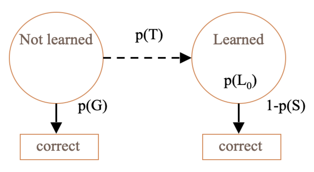
Learning Parameters
Two Learning Parameters
- p(L0). Probability the skill is already known before the first opportunity to use the skill in problem solving.
- p(T). Probability the skill will be learned at each opportunity to use the skill.

Performance Parameters
Two Performance Parameters
- p(G). Probability the student will guess correctly if the skill is not known.
- p(S). Probability the student will slip (make a mistake) if the skill is known.

Performance Parameters
Two Performance Parameters
- p(G). Probability the student will guess correctly if the skill is not known.
- p(S). Probability the student will slip (make a mistake) if the skill is known.

Comments? Questions?
Predicting Current Student Correctness
PCORR = P(Ln)P(S)+P(~Ln)P(G)
Bayesian Knowledge Tracing
Whenever the student has an opportunity to use a skill
The probability that the student knows the skill is updated
Using formulas derived from Bayes’ Theorem
Formulas
\[ P(L_{n-1}|Correct_{n}) = \frac{P(L_{n-1})*(1-P(S))}{P(L_{n-1})*(1-P(S))+(1-P(L_{n-1}))*P(G)} \\\\\\ P(L_{n-1}|Incorrect_{n}) = \frac{P(L_{n-1})*(P(S))}{P(L_{n-1})*(P(S))+(1-P(L_{n-1}))*(1-P(G))} \\\\\\ P(L_{n}|Action_{n}) = P(L_{n-1}|Action_{n}) +(1- P(L_{n-1}|Action_{n}) * p(T)) \]
Example
P(L0) = 0.4, P(T) = 0.1, P(S) = 0.3, P(G) = 0.2
| Actual | P(Ln-1) | P(Ln-1|actual) | P(Ln) |
|---|---|---|---|
| 0.4 | |||
Example
P(L0) = 0.4, P(T) = 0.1, P(S) = 0.3, P(G) = 0.2
| Actual | P(Ln-1) | P(Ln-1|actual) | P(Ln) |
|---|---|---|---|
| 0 | 0.4 | \[ \frac{(0.4)(0.3)}{(0.4)(0.3)+(0.6)(0.8)} \] | |
| . | |||
| . | |||
| . |
Example
P(L0) = 0.4, P(T) = 0.1, P(S) = 0.3, P(G) = 0.2
| Actual | P(Ln-1) | P(Ln-1|actual) | P(Ln) |
|---|---|---|---|
| 0 | 0.4 | \[ \frac{(0.12)}{(0.12)+(0.48)} \] | |
| . | |||
Example
P(L0) = 0.4, P(T) = 0.1, P(S) = 0.3, P(G) = 0.2
| Actual | P(Ln-1) | P(Ln-1|actual) | P(Ln) |
|---|---|---|---|
| 0 | 0.4 | 0.2 | |
Before we knew they got it wrong, we thought they had a 40% chance of knowing it. But after they get it wrong, we have a 20% chance that they know it. They still might have slipped.
Example
P(L0) = 0.4, P(T) = 0.1, P(S) = 0.3, P(G) = 0.2
| Actual | P(Ln-1) | P(Ln-1|actual) | P(Ln) |
|---|---|---|---|
| 0 | 0.4 | 0.2 | 0.2+(0.8)(0.1) |
The probability that they know it afterward is the probability that they knew it plus the probability they didn’t know it times the probability they learned it.
Example
P(L0) = 0.4, P(T) = 0.1, P(S) = 0.3, P(G) = 0.2
| Actual | P(Ln-1) | P(Ln-1|actual) | P(Ln) |
|---|---|---|---|
| 0 | 0.4 | 0.2 | 0.28 |
And that is 0.28
Example
P(L0) = 0.4, P(T) = 0.1, P(S) = 0.3, P(G) = 0.2
| Actual | P(Ln-1) | P(Ln-1|actual) | P(Ln) |
|---|---|---|---|
| 0 | 0.4 | 0.2 | 0.28 |
| 0.28 | |||
The probability that they know it afterward is the probability that they knew it before the second action.
Example
P(L0) = 0.4, P(T) = 0.1, P(S) = 0.3, P(G) = 0.2
| Actual | P(Ln-1) | P(Ln-1|actual) | P(Ln) |
|---|---|---|---|
| 0 | 0.4 | 0.2 | 0.28 |
| 1 | 0.28 | ||
If the student gets the action right.
Example
P(L0) = 0.4, P(T) = 0.1, P(S) = 0.3, P(G) = 0.2
| Actual | P(Ln-1) | P(Ln-1|actual) | P(Ln) |
|---|---|---|---|
| 0 | 0.4 | 0.2 | 0.28 |
| 1 | 0.28 | \[ \frac{(0.28)(0.7)}{(0.28)(0.7)+(0.72)(0.2)} \] | |
If the student gets the action right. In that case, the probability they knew it before they got it right is the probability they had known it times hadn’t slipped. Over that probability, plus the probability that they didn’t know it and they guessed.
Example
P(L0) = 0.4, P(T) = 0.1, P(S) = 0.3, P(G) = 0.2
| Actual | P(Ln-1) | P(Ln-1|actual) | P(Ln) |
|---|---|---|---|
| 0 | 0.4 | 0.2 | 0.28 |
| 1 | 0.28 | \[ \frac{(0.196)}{(0.196)+(0.144)} \] | |
Please move on to next slide
Example
P(L0) = 0.4, P(T) = 0.1, P(S) = 0.3, P(G) = 0.2
| Actual | P(Ln-1) | P(Ln-1|actual) | P(Ln) |
|---|---|---|---|
| 0 | 0.4 | 0.2 | 0.28 |
| 1 | 0.28 | 0.58 | |
That turns into .58.
When they got it wrong, they went down from .4 to .2, which came up to .28, and then that .28 after they got it right was reassessed to be .58. These are pretty big changes and that’s because the probabilities of slip and guess are pretty low on this model.
Example
P(L0) = 0.4, P(T) = 0.1, P(S) = 0.3, P(G) = 0.2
| Actual | P(Ln-1) | P(Ln-1|actual) | P(Ln) |
|---|---|---|---|
| 0 | 0.4 | 0.2 | 0.28 |
| 1 | 0.28 | 0.58 | (0.58) + (0.42)(0.1) |
So then the probability that they knew it afterward is the probability that they knew it beforehand, plus the probability that they didn’t know it times the probability they learned it,
Example
P(L0) = 0.4, P(T) = 0.1, P(S) = 0.3, P(G) = 0.2
| Actual | P(Ln-1) | P(Ln-1|actual) | P(Ln) |
|---|---|---|---|
| 0 | 0.4 | 0.2 | 0.28 |
| 1 | 0.28 | 0.58 | 0.62 |
which comes out to .62.
Your Turn
P(L0) = 0.4, P(T) = 0.1, P(S) = 0.3, P(G) = 0.2
| Actual | P(Ln-1) | P(Ln-1|actual) | P(Ln) |
|---|---|---|---|
| 0 | 0.4 | 0.2 | 0.28 |
| 1 | 0.28 | 0.58 | 0.62 |
| 1 |
Comments? Questions?
Conceptual Idea Behind Knowledge Tracing
Parameter Constraints
Typically, the potential values of BKT parameters are constrained
To avoid model degeneracy
Typically the potential values of BKT parameters are constrained.
The guess and slip we had are kind of low, so the model is fairly dynamic. However, we want to constrain those values somewhat to avoid what’s called model degeneracy, which is based on violating the conceptual idea behind knowledge tracing.
Conceptual Idea Behind Knowledge Tracing
Knowing a skill generally leads to correct performance
Correct performance implies that a student knows the relevant skill
Hence, by looking at whether a student’s performance is correct, we can infer whether they know the skill
That conceptual idea is that knowing a skill generally leads to correct performance, and correct performance implies that a student knows the relevant skill. So, the idea is that by looking at whether a student’s performance is correct, we can infer whether they know the skill.
Essentially
- A knowledge model is degenerate when it violates this idea
- When knowing a skill leads to worse performance
- When getting a skill wrong means you know it
Essentially, a knowledge model is degenerate when it violates this idea. Knowing a skill leads to worse performance, and getting a skill wrong means that you know it. It’s weird, right? That’s why it’s called a degenerate model. Different people have proposed some constraints.
Parameter Constraints Proposed
Beck
- P(G)+P(S)<1.0
R. S. d. Baker, Corbett, and Aleven (2008):
- P(G)<0.5, P(S)<0.5
Corbett and Anderson (1995)
- P(G)<0.3, P(S)<0.1
Joe Beck has proposed that the probability of guessing plus the probability of slip must be less than 1.
Baker, Corbin, and Alavin have proposed that guess and slip each have to be less than 0.5.
Corbin and Anderson originally proposed, and this was not entirely just for model degeneracy but also based on some theorizing about what was probable, that P of G has to be less than 0.3 and P of S has to be less than 0.1.
Baker would say that when either guess or slip gets above 0.5, you’re in a situation where the behavior doesn’t mean what it looks like.
Beck would say that for some cases where the modeling can get difficult, specifically like with automated speech responses where you’re making inferences, there might be enough error that you might get a guess or slip above 0.5. But as long as they’re under 1.0 as a sum, it’s still okay.
Knowledge Tracing
How do we know if a knowledge tracing model is any good?
Our primary goal is to predict knowledge
How do we know if a knowledge tracing model is any good beyond whether it is degenerate or not? The primary goal is to predict knowledge,
Knowledge Tracing
How do we know if a knowledge tracing model is any good?
Our primary goal is to predict knowledge
- But knowledge is a latent trait
- So we instead check our knowledge predictions by checking how well the model predicts performance
but knowledge is a latent trait. So, instead, we check our knowledge predictions by checking how all the models predict performance.
Fitting a Knowledge-Tracing Model
In principle, any set of four parameters can be used by knowledge-tracing
But parameters that predict student performance better are preferred
In principle, any set of four parameters can be used by knowledge tracing. However, parameters that predict student performance better are preferred.
Knowledge-Tracing
So, we pick the knowledge tracing parameters that best predict performance
Defined as whether a student’s action will be correct or wrong at a given time
So we try to pick the knowledge-tracing parameters that best predict performance. That is, whether a student’s action will be correct or wrong at a given time when knowledge tracing predicts it will be.
Are these the same thing?
Predicting performance on next attempt
Inferring latent knowledge
What are some alternate ways to assess
- Whether a model is successful at inferring latent knowledge
What are some alternate ways to assess
Whether a model is successful at inferring latent knowledge
Why aren’t those approaches used more often?
Comments? Questions?
Questions?
Fitting a Knowledge-Tracing Model
Fitting a Knowledge-Tracing Model
In principle, any set of four parameters can be used by knowledge-tracing
But parameters that predict student performance better are preferred
In principle, any set of four parameters can be used by knowledge-tracing.
But parameters that predict student performance better are preferred.
Fit Methods
I could spend an hour talking about the ways to fit Bayesian Knowledge Tracing models.
Three Public Tools
hmmsclbl
BNT-SM: Bayes Net Toolkit – Student Modeling
- http://www.cs.cmu.edu/~listen/BNT-SM/
BKT-BF: BKT-Brute Force (Grid Search)
https://learninganalytics.upenn.edu/ryanbaker/BKT-BruteForce.zipPython Grid Search (slower than BKT-BF)
- https://github.com/ChNabil/BKT_python_gridsearch
There are three public tools you can use to fit BKT parameters:
HMMSCLBL by Michael Yudelson..
BNT-SM, the Bayes Net Toolkit Student Modeling, which does expectation maximization
BKTBF, BKT Brute Force, which does a grid search algorithm.
All three of these are open on the web, and you can use them, they’re all fine really and work approximately equally well.
Which one should you use?
They’re all fine – they work approximately equally well
My group uses BKT-BF to fit Classical BKT and BNT-SM to fit variant models
But some commercial colleagues use Fit BKT at Scale
All three of these are open on the web, and you can use them, they’re all fine really and work approximately equally well.
Note…
- The Equation Solver in Excel replicably does worse for this problem than these packages
The one thing you shouldn’t do is to use the Excel equation solver. That replicably does worse for the problem than these packages. So use some existing package - they’re out there.
How much data do you need? Slater and Baker (2018)
- Depends on your goal
Predict student mastery, if ok to be off by 2-3 problems:
- As few as 25 students and 3 problems apiece, if P(T) values are low
Predict student mastery, if higher precision desired:
- 250 students and 3 problems apiece
Make inferences about model parameter values (for example, to identify skills that need to be fixed)
- 250 students and 6 problems apiece
One common practical question that people ask is:
how much data you need to fit BKT.
The answer depends on your goal. As Slater and Baker’s large-scale simulation study showed, if you’re intending to predict student mastery, and it’s ok for the system to decide the student has mastered two or three problems too early or too late, you can get away with as few as 25 students and 3 problems per skill, as long as P(T) values are low. If you do this, and see high P(T) values, you might need to get more data. If you want high precision on exactly when the student mastered, you might want to go as high as 250 students, but 3 problems per student is still generally OK. A harder task is making inferences about model parameter values. You might do this if, for example, you want to find skills with really high slip or guess rates, to fix them. In this case, you need 250 students and 6 problems per student.
BKT: Core Uses
Mastery learning
Reports to teachers on student skill
The two core uses of BKT are, of course:
supporting mastery learning – determining when a student has mastered a skill in order to advance them
and providing reports to teachers (or the student themself) on what skills the student has and hasn’t yet mastered.
BKT: Extended Uses
Use in behavior detectors (such as gaming the system)
Use to identify problematic skills for re-design (with very high slip or guess or initial knowledge)
Use in discovery with models analyses (such as correlating student in-platform learning to test scores)
But there are several other common uses as well, including using BKT estimates as components in behavior detectors, like gaming the system, or identifying skills with very high slip or guess or initial knowledge, to drive iterative improvement of the learning system, or in variables in various kinds of analyses, like correlation students’ performance and learning within a learning platform, to external measures like their test scores.
BKT: Extended Uses
Conditionalizing P(T)
There have been a bunch of extensions to BKT. It’s not just a good model, it’s also been the basis for a lot of other interesting work.
BKT: Extended Uses
Moment-by-moment learning estimation
(calculating P(T) in specific step)Which moment-by-moment learning curves are associated with more robust learning? (Ryan S. Baker et al. (2013))
What behaviors predict “eureka” moments (Moore, Baker, and Gowda (2015))
Which types of content are associated with more learning? (Slater et al. (2016))
Some examples here, they will be introduced later in Advanced BKT part.
BKT: Extended Uses
Detecting carelessness (contextual slip)
(calculating P(S) in specific step)Predicts test score (Pardos et al. (2014)), college enrollment (M. O. Pedro et al. (2013)), job several years later (Almeda and Baker (2020))
Some examples here, they will be introduced later in Advanced BKT part.BKT: Extended Uses
BKT: Extended Uses
Transfer assessment
(adding P(T) from other skills)Used to study relationship between skills (M. S. Pedro et al. (2014))
Including in graduate students learning research skills across several years (Kang et al. (2022))
Some examples here, they will be introduced later in Advanced BKT part.BKT: Extended Uses
Further Discussion
How can you apply these methods to your own research or practice?
DISCUSSION:
- How can you apply these methods to your own research or practice?
What’s NEXT?
Complete the ASSISTments activity: [insert link here]
Complete the badge requirement document: [insert link here]
Thank you! Any questions?
What’s next?
- assignments
More Detail on Advanced BKT
More Detail on Advanced BKT
BKT has strong assumptions
One of the key assumptions is that parameters vary by skill, but are constant for all other factors
What happens if we remove this assumption?
Modifying the assumptions of Bayesian knowledge tracing:
- BKTS has strong assumptions. One key assumption is that parameters vary by skill but are constant for all other factors. What happens if we remove this assumption?
BKT with modified assumptions
Conditionalizing Help or Learning
Contextual Guess and Slip
Moment by Moment Learning
Modeling Transfer Between Skills
If we remove any of those assumptions, we get different kinds of algorithms that can be used for different purposes, like algorithms for conditionalizing help or learning, algorithms for contextual guess and slip, moment-by-moment learning models, and algorithms that can model the transfer between skills.
Beck, Chang, Mostow, & Corbett 2008
Beck, J.E., Chang, K-m., Mostow, J., Corbett, A. (2008) Does Help Help? Introducing the Bayesian Evaluation and Assessment Methodology. Proceedings of the International Conference on Intelligent Tutoring Systems.
![]()
Now let’s first discuss Beck’s help model.
Notes
In this model, help use is not treated as direct evidence of not knowing the skill
Instead, it is used to choose between parameters
Makes two variants of each parameter
One assuming help was requested
One assuming that help was not requested
In this model, help use is not treated as direct evidence of not knowing the skill, unlike classical BKT, but instead, it’s used to choose between parameters. This model makes two variants of each parameter, one of them assuming help was requested and one of them assuming that help was not requested.
Beck, et al.’s (2008) Help Model
%20Help%20Model.png)
This model otherwise looks just like BKT, at every single parameter, there are two variants of it, a given help, a given H, and a given not help, given not H. This gives us eight parameters per skill: the four classical parameters times two.
Beck, et al.’s (2008) Help Model
- Parameters per skill: 8
- Fit using Expectation Maximization
- Takes too long to fit using Grid SearchIt fits using expectation maximization because it takes too long to fit using brute force. Brute Force works when we’ve got an N to the fourth problem, but it doesn’t work so well for an N to the eighth problem.
Beck, et al.’s (2008) Help Model
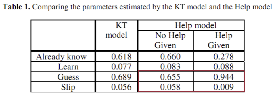
In his original paper, he found that there were fairly different parameter values for guess and slip based on whether or not the person asked for help.
Beck, et al.’s (2008) Help Model
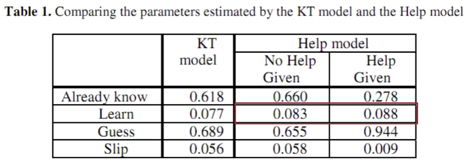
(Explaining about the difference)
Notes
This model did not lead to better prediction of student performance
But useful for understanding effects of help
It’s worth noting that:
this model didn’t lead to a better prediction of student performance, but it was useful for understanding the effects of help. One thing about BKT that’s noteworthy is that a lot of the modern extensions of BKT actually aren’t about fitting the data better.
A lot of the things that BKT can do for you have to do not with getting slightly better prediction of next problem correctness, but with being able to infer other things.
BKT with modified assumptions
Conditionalizing Help or Learning
Contextual Guess and Slip
Moment by Moment Learning
Modeling Transfer Between Skills
The 2nd modification of assumptions of BKT is contextual guess and slope.
Contexual Guess-and-Slip
Baker, R.S.J.d., Corbett, A.T., Aleven, V. (2008) More Accurate Student Modeling Through Contextual Estimation of Slip and Guess Probabilities in Bayesian Knowledge Tracing. Proceedings of the 9th International Conference on Intelligent Tutoring Systems, 406-415.
![]()
The 2nd modification of assumptions of BKT is contextual guess and slipe.
Contexual Guess-and-Slip
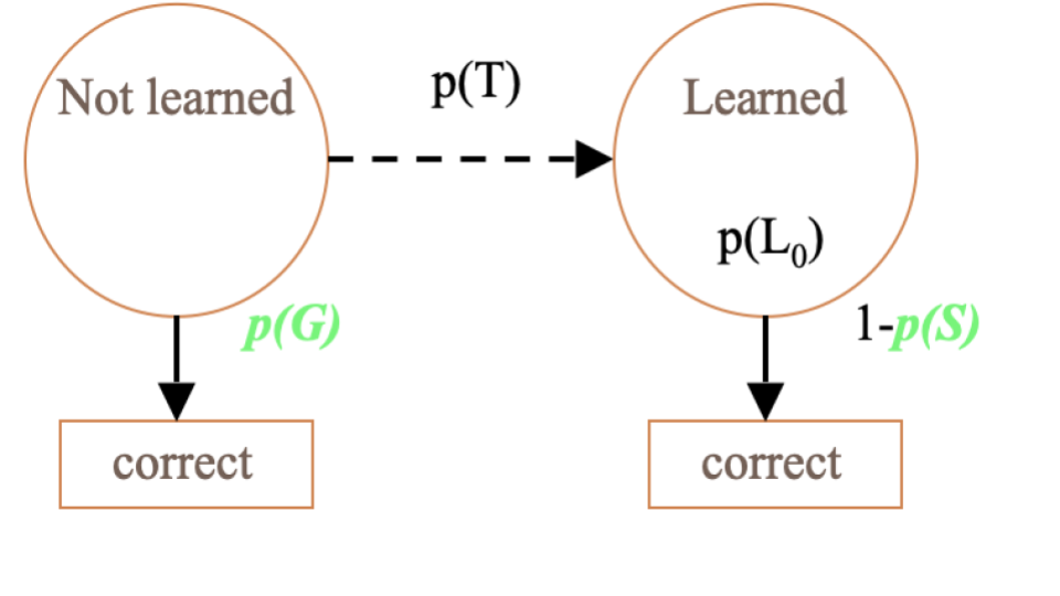
In this model, we have the exact same L0, T, G, and S, but the G and S aren’t parameters per skill. They’re models.
Contexual Slip: The Big Data
Why one parameter for slip
- For all situations
- For each skillWhen we can have a different prediction for slip
For each situation
Across all skills
The big idea is why one parameter for slip for all situations for each skill when we can have a different prediction for slip for each situation across all skills.
In other words
- P(S) varies according to context
For example
Perhaps very quick actions are more likely to be slips
Perhaps errors on actions which you’ve gotten right several times in a row are more likely to be slips
In other words, P of S varies according to context.
- Example: perhaps very quick actions are more likely to be slips, or perhaps errors in actions that you’ve gotten right several times in a row are more likely to be slips.
Contexual Guess and Slip Model
Guess and slip fit using contextual models across all skills
Parameters per skill: 2 + (P (S) model size)/skills + (P (G) model size)/skills
Guess and slip are therefore fit using contextual models across all skills.
In this case, the parameters per skill are 2 plus the model size of P of S divided by the number of skills plus the guess model size divided by skills. This ends up amortizing to a good bit less than four parameters per skill.
How are these models developed?
Take an existing skill model
Label a set of actions with the probability that each action is a guess or slip, using data about the future
- Use these labels to machine-learn models that can predict the probability that an action is a guess or slip, without using data about the future
- Use these machine-learned models to compute the probability that an action is a guess or slip, in knowledge tracing
How are these models developed?
We take an existing skill model, and label a set of actions with the probability that each action is a guess or a slip using data about the future. We’re going to use the data about the future, but we’re not actually going to use it in the running model.
We use these labels to machine learning models that can predict the probability that an action is a guess or a slip without using data about the future.
We then use these machine learning models to compute the probability that an action is a guess or a slip in real-time knowledge tracing.
Again, we’re using the future to build the models, but we’re not using the future to actually run the models.
How are these models developed?
2. Label a set of actions with the probability that each action is a guess or slip, using data about the future
Predict whether action at time N is guess/slip
Using data about actions at time N+1, N+2
This is only for labeling data! @
Not for use in the guess/slip models
More specifically, we label a set of actions with the probability that each action is a guess or a slip using data about the future. Predict whether an action at a time is a guess or a slip using data about the actions at time n plus 1 and n plus 2.
How are these models developed?
2. Label a set of actions with the probability that each action is a guess or slip, using data about the future
The intuition:
If action N is right
And actions N+1, N+2 are also right
- It’s unlikely that action N was a guess
If actions N+1, N+2 were wrong
- It becomes more likely that action N was a guess
I’ll give an example of this math in few minutes…
The intuition is that if action n is right and actions n plus 1 and n plus 2 were also right, it’s probabilistically unlikely that action n was a guess because the probability that you’d get three things right in a row by guessing is just really infinitesimal. Similarly, if actions n plus 1 and n plus 2 were wrong, it becomes more likely that action n was a guess.
How are these models developed?
3. Use these labels to machine-learn models that can predict the probability that an action is a guess or slip
Features distilled from logs of student interactions with tutor software
Broadly capture behavior indicative of learning
Having gotten these labels, we then use them to machine-learn models that can predict the probability that an action is a guess or a slip. We take features distilled from logs of student interactions of the tutor software that broadly capture behavior indicative of learning.
- Baker-Corbinolev 2008, it selected these from the same set of initial features previously used in detectors of gaming a system and off-task behavior.
How are these models developed?
3. Use these labels to machine-learn models that can predict the probability that an action is a guess or slip
Linear regression
- Did better on cross-validation than fancier algorithms
One guess model
One slip model
In the first work, we used linear regression, which, in this early work, did better on cross-validation than fancier algorithms. One guess model, one slip model.
How are these models developed?
4. Use these machine-learned models to compute the probability that an action is a guess or slip, in knowledge tracing
Within Bayesian Knowledge Tracing
Exact same formulas
Just substitute a contextual prediction about guessing and slipping for the prediction-for-each-skill
Having these probabilities, we just plug the estimates, the numbers, into Bayesian knowledge tracing, the exact same formulas as before. We’re just substituting a contextual prediction about guessing and slipping for the prediction for each skill.
BKT with modified assumptions
Conditionalizing Help or Learning
Contextual Guess and Slip
Moment by Moment Learning
Modeling Transfer Between Skills
A third way to modify BKT’s assumptions:
- moment-by-moment learning.
Moment-by-Moment Learning Model
Baker, R.S.J.d., Goldstein, A.B., Heffernan, N.T. (2011) Detecting Learning Moment-by-Moment. International Journal of Artificial Intelligence in Education, 21 (1-2), 5-25.

A third way to modify BKT’s assumptions:
- moment-by-moment learning.
Moment-by-Moment Learning Model (Baker, Goldstein, & Heffernan, 2010)
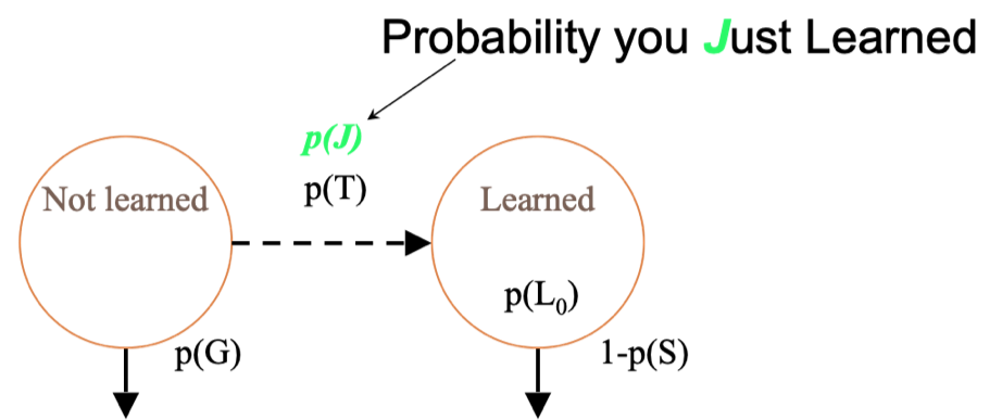
The moment-by-moment learning model, as published, uses Bayesian knowledge tracing and doesn’t try to substitute any of the four parameters. It just adds a variant parameter for P of T, the probability you just learned. That’s not quite the same as P of T.
P(J)
P(T) = chance you will learn if you didn’t know it
P(J) = probability you Just Learned
- P(J) = P(~Ln ^ T)
P of T is the chance you’re going to learn if you didn’t know it already. P of J is the probability you just learned. In other words, it’s the probability that you didn’t know it and then you learned it. Not quite the same thing, although it’s quite related.
P(J) is distinct from P(T)
%20is%20distinct%20from%20P(T).png)
When say P of J is distinct from P of T, they can have values that are quite different.
Example: the difference between a probability of T of 0.6 in the context where you have an initial probability of knowing it of 0.1 or 0.96. If you had a 10% chance of knowing it and you have a 60% chance of learning it if you didn’t know it, the probability you just learned is 54%.
That’s a lot of learning
That’s learning. But if your probability of knowing it to begin with was 96% and you had a 60% chance of learning it, you only have a 2% chance that you just learned it. That’s not very much learning.
Labeling P(J)
Based on this concept:
- “The probability a student did not know a skill but then learns it by doing the current problem, given their performance on the next two.”
P(J) = P(~Ln ^ T | A+1+2 )
*For full list of equations, see
Ryan SJD Baker, Goldstein, and Heffernan (2011)
P of J is labeled based on the concept. It’s very similar to the contextual guess and slip model. The probability a student doesn’t know a skill but then learns it by doing the current problem given their performance on the next two.
Breaking down P(~Ln ^ T | A+1+2 )

We can calculate the probability that they didn’t know it and they learned it from those next two actions with an application of Bayes’ theorem. We say the probability they didn’t know it and learned it given the next two actions is the probability of those next two actions given that they didn’t know it and they learned it times the probability that in general, regardless of those two actions, they didn’t know it and they learned it over the probability of those next two actions across all contexts.
Breaking down P(A+1+2 | Ln) P(Ln): One example
P(A+1+2 = C, C | Ln ) = P(~S)P(~S)
P(A+1+2 = C, ~C | Ln ) = P(~S)P(S)
P(A+1+2 = ~C, C | Ln ) = P(S)P(~S)
P(A+1+2 = ~C, ~C | Ln ) = P(S)P(S)

Example:
What about the probabilities of the next two actions, given that they knew it, times the probability that they knew it? Well, there are only 4 possibilities for those two actions.
Correct, correct.
Correct, not correct.
Not correct, correct.
And not correct, not correct.
And those turn out to be if you knew it, the probability of correct, correct if you knew it is the probability you didn’t slip, times the probability you didn’t slip.
The probability that you got it wrong and then right if you knew it was the probability you didn’t slip, times the probability you slipped, and so on.
This case is going to be more complicated for the case that you didn’t know it and you didn’t learn it because in that case, we’re trying to estimate the probability as we go forward based on the possibility that you may have learned it or not between the first and second attempts. So, the equations get really complicated at this point.
Features of P(J)
Distilled from logs of student interactions with tutor software
Broadly capture behavior indicative of learning
Now P of J, like contextual P of S and G, we took features distilled from logs of student interactions with tutor software that broadly captured behaviors indicative of learning. These features were selected from the same initial set of features previously used in detectors of gaming the system, off-task behavior, and carelessness, aka the probability of contextual slip.
Features of P(J)
- All features use only first response data
- Later extension to include subsequent responses only increased model correlation very slightly – not significantly
All the features in the original work used only first response data. Later extensions to include subsequent responses only increased the model correlation very slightly, not statistically significantly.
Uses
Patterns in P(J) over time can be used to predict whether a student will be prepared for future learning (Hershkovitz et al. (2013), Ryan S. Baker et al. (2013)) and standardized exam scores (Jiang et al. (2015))
P(J) can be used as a proxy for Eureka moments in Cognitive Science research (Moore, Baker, and Gowda (2015))
We then had a model that we could use for a few things.
We’re not using this model at any point to try to improve our prediction of student performance in the system. Instead, we’re looking at how we can use this in analysis. It turns out that patterns in P of J over time can be used to predict whether theit’s student is prepared for future learning:.
when they encounter the first piece of curriculum material beyond this current system can they actually learn from it and do well on a test. Patterns of P of J during the use of the system turn out to be predictive of this. Also, it turns out that P of J over time can be used to predict standard as exam scores.
in a third recent use, P of J can be used as a proxy for eureka moments in cognitive science research. We can look for moments where students had spectacularly high learning, say higher than 99 percent of all learning episodes, and say what distinguishes the behavior that precedes this.
Alternate Method
Assume at most one moment of learning
Try to infer when that single moment occurred, across entire sequence of student behavior
Some good theoretical arguments for this – more closely matches assumptions of BKT
Has not yet been studied whether this approach has same predictive power as P(~Ln ^ T | A+1+2 ) method
There is an alternate method for calculating P of J:
we assume at most one moment of learning, and then we try to infer when that single moment occurred across the entire sequence of student behavior. This was done both by Van de Sande (2013) and by Pardos & Yudelson (2013). There are some good theoretical reasons why you might want to do this. It actually more closely matches the assumptions of BKT.
Is it better? We don’t know yet.
Although there have been a couple of papers on it, we haven’t yet seen anyone study whether this approach has the same predictive power as the method from Baker-Goldstein-Heffernan for things like predicting preparation for future learning. Stairway as the exam scores or Eureka moments.
BKT with modified assumptions
Conditionalizing Help or Learning
Contextual Guess and Slip
Moment by Moment Learning
Modeling Transfer Between Skills
A fourth type of modifying the assumption of BKT is modeling transfer between skills.
This is unlike the other three, for which we’re still looking within a skill essentially, even though some of the variants in contextual guessing slip vary by skill.
This one actually says what if we relax the assumption that each skill is independent from every other skill?
Modeling Transfer Between Skills
Sao Pedro, M., Jiang, Y., Paquette, L., Baker, R.S., Gobert, J. (2014) Identifying Transfer of Inquiry Skills across Physical Science Simulations using Educational Data Mining. Proceedings of the 11th International Conference of the Learning Sciences.

The first paper on this comes from Sao Pedro and colleagues in 2014, and what this model did was it said as follows:
How this model works
- Classic BKT: Separate BKT model for each skill
BKT-PST (Partial Skill Transfer) M. S. Pedro et al. (2014): Each skill’s model can transfer in information from other skills
BKT-PST: One time (when switching skill)
BKT-PSTC Kang et al. (2022): At each time step
Classic BKT said says that there would will be a separate BKT model for each skill. BKT-PST partial skill transfer says instead that each skill model can transfer information from other skills, and in its original formulation in 2014, this happened exactly once when switching between skills in a system. But in Kang et al., in 2022 said wait a minute sometimes you switch back and forth between skills. So in that case we’re going to do it at each time step.
BKT-PST/PSTC Model
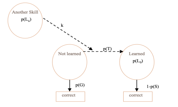
The BKT PST or PSTC model is basically the original BKT graph, which you see at the bottom. But then from some other skill, there’s a transfer in which has parameter K. This method of transferring information between skills hasn’t been used a ton but it has been used by Sale Pedro and colleagues to study the relationship between skills in a science simulation.
Uses
Used to study relationship between skills in science simulation
( M. S. Pedro et al. (2014))
Used to study which research skills help graduate students learn other research skills, across several years (Kang et al. (2022))
Specifically, if you master skill A are you starting off better in skill B. Kang and her colleagues used it to study which research skills help graduate students learn other research skills across several years. In that case every year the grad student might be getting better in each of several research skills, and the question is if they acquire skill A in year N are they better at skill B in your N plus one?
Uses
Contextualization approaches do not appear to lead to overall improvement on predicting within-tutor performance
But they can be useful for other purposes
Predicting robust learning
Understanding learning better
Understanding relationships between skills
Overall, across all four of these types of examples, contextualization approaches generally don’t appear to lead to big overall improvements in predicting xatutor performance (see Gonzales-Brenes et al., 2014). But in general, they’re really good for other purposes, like predicting robust learning, understanding learning better, and understanding the relationship between the skills.
There are a lot of utilities to modifying the assumptions of BKT that are harder with some of the more contemporary algorithms which is one of the reasons why researchers still sometimes use BKT.
Thank you!


Comments or Questions?