ENA and Virtual Internship Conversations

TM Module 3: Case Study Key

Author

Dr. Shaun Kellogg

Published

July 13, 2025

0. INTRODUCTION

This case study extends the methodology presented in the Learning Analytics in STEM Education Research (LASER) Institute by demonstrating the application of Epistemic Network Analysis (ENA) to explore collaborative learning processes in digital STEM education environments. ENA is a sophisticated technique that visualizes and quantifies connections among concepts in coded data, offering rich insights into how learners construct knowledge collaboratively.

Epistemic Network Analysis, developed by David Williamson Shaffer and colleagues, enables researchers to analyze discourse and interactions within learning communities, revealing the patterns of connections among key elements of the learning process. The method is particularly valuable in STEM education research, where understanding complex interactions is critical for improving learning outcomes and pedagogical practices.

Case Study Focus

This case study is adapted from a chapter by Tan et al. Tan et al. (2024) in the excellent book, Learning Analytics Methods and Tutorials. Our focus will be on applying ENA to investigate discourse patterns in a collaborative digital STEM learning environment. Specifically, we will examine how participants engage in problem-solving activities, make connections between STEM concepts, and collaboratively construct knowledge.By using ENA, researchers can systematically map the epistemic frames that occur when learners collaboratively tackle STEM-related problems, providing a quantitative yet qualitative-rich understanding of group learning dynamics. This analysis is particularly critical for understanding the nuances of learner interactions in digital environments, which often involve complex dialogues and exchanges that traditional qualitative methods might miss or oversimplify.

Our ENA case study covers the following concepts and skills:

  1. Prepare. In the Prepare phase, we familiarize ourselves with the context of our case study, which leverages data from virtual internships aimed at enhancing engineering design thinking. We define specific research questions guided by prior studies and set up our analytical environment by loading essential R packages needed for our analyses, including {tidyverse}, {tidytext}, and {rENA}.

  2. Wragle. In the Wrangle phase, we carefully import, organize, and prepare our data for analysis. This involves importing text-based discourse data from the RescuShell internship, specifying critical parameters for the ENA model (such as units of analysis, qualitative coding schemes, conversational boundaries, window size for capturing interactions, and group definitions), and finally constructing an ENA model object that captures our data’s structure and interaction patterns.

  3. Explore. In the Explore phase, we use both visual and numeric methods to deeply investigate and interpret our ENA model. We create visual summaries of key model outputs, plotting mean networks and identifying meaningful differences across groups. We also provide numeric summaries of connection counts, normalized line weights, and ENA points to further understand underlying quantitative patterns that shape our visualizations.

  4. Model In the Model phase, we conduct rigorous statistical analyses to validate and interpret the patterns observed in the visual and numeric explorations. We perform comparative statistical tests (such as t-tests and Mann-Whitney U tests) to evaluate differences in epistemic network structures between novice and expert learner conditions. Additionally, we evaluate model quality through variance explained, goodness-of-fit statistics, and interpretive validation (closing the interpretative loop) to ensure robust and meaningful results.

  5. Communication. Finally, in the Communicate phase, we synthesize and clearly articulate our key findings, selecting the most meaningful insights to share with broader audiences. We focus on translating complex analyses into actionable insights through polished data visualizations and narrative explanations that align closely with our original research questions.

1. PREPARE

To help us better understand the context, questions, and data sources we’ll be using in Module 3, this section will focus on the following topics:

  1. Context. As context for our analysis this week, we’ll review an article by Arastoopour et al. Arastoopour Irgens et al. (2015) that uses ENA to explore virtual internships as one method for teaching engineering design thinking.
  2. Questions. We’ll also examine what insight topic modeling can provide to a question that we asked participants to answer in their professional learning teams (PLTs).
  3. Project Setup. This should be very familiar by now, but we’ll also learn about load the required packages for the topic modeling case study.

1a. Context

Arastoopour Irgens, G., Shaffer, D. W., Swiecki, Z., Ruis, A. R., & Chesler, N. C. (2015). [Teaching and assessing engineering design thinking with virtual internships and epistemic network analysis](https://open.clemson.edu/cgi/viewcontent.cgi?article=1004&context=ed_human_dvlpmnt_pub). International Journal of Engineering Education.

Arastoopour Irgens, G., Shaffer, D. W., Swiecki, Z., Ruis, A. R., & Chesler, N. C. (2015). [Teaching and assessing engineering design thinking with virtual internships and epistemic network analysis](https://open.clemson.edu/cgi/viewcontent.cgi?article=1004&context=ed_human_dvlpmnt_pub). International Journal of Engineering Education.

Abstract

An engineering workforce of sufficient size and quality is essential for addressing significant global challenges such as climate change, world hunger, and energy demand. Future generations of engineers will need to identify challenging issues and design innovative solutions. To prepare young people to solve big and increasingly global problems, researchers and educators need to understand how we can best educate young people to use engineering design thinking. In this paper, we explore virtual internships, online simulations of 21st-century engineering design practice, as one method for teaching engineering design thinking. To assess the engineering design thinking, we use epistemic network analysis (ENA), a tool for measuring complex thinking as it develops over time based on discourse analysis. The combination of virtual internships and ENA provides opportunities for students to engage in authentic engineering design, potentially receive concurrent feedback on their engineering design thinking, and develop the identity, values, and ways of thinking of professional engineers.

Data Source & Analysis

Interaction data were collected from RescuShell, an engineering virtual internship platform. This digital platform provides a realistic engineering context where learners collaborate in solving authentic problems, simulating tasks common to engineering practice. The data used in this case study were previously examined by Shaffer & Arastoopour (2014), Arastoopour et al. (2016), and Chesler et al. (2015). The data consist primarily of text-based interactions recorded in discussion forums, chat logs, and collaborative workspaces within RescuShell.

For further details regarding data collection and analysis of these data sources, see also the following papers:

  • Shaffer, D. W., & Arastoopour, G. (2014). Epistemic network analysis of engineering virtual internships. Journal of Engineering Education, 103(4), 625-651.

  • Arastoopour, G., Shaffer, D. W., Chesler, N. C., & Linderoth, J. (2016). Epistemic network analysis as a measure of critical thinking in engineering education. International Journal of Engineering Education, 32(6), 2476-2486.

  • Chesler, N. C., Arastoopour, G., D’Angelo, C. M., Bagley, E. A., & Shaffer, D. W. (2015). Design of professional practice simulator for educating and motivating first-year engineering students. Advances in Engineering Education, 4(2), 1-27.

Summary of Key Findings

The following highlights key findings related to the discourse and interactions in engineering virtual internships:

  • ENA effectively identified distinct discourse patterns among learners participating in engineering virtual internships, highlighting how knowledge was co-constructed and shared within these collaborative spaces.

  • Analysis demonstrated how learners’ epistemic networks evolved significantly as they engaged in iterative problem-solving activities, with certain key concepts becoming increasingly central as students collaboratively advanced through the internship challenges.

  • Results indicated that the discourse patterns identified by ENA corresponded to deeper cognitive engagement, where students actively negotiated and co-constructed engineering knowledge rather than merely exchanging surface-level information.

  • Findings from prior analyses underscore the utility of ENA in capturing nuanced learner interactions and in differentiating between various collaborative learning approaches, suggesting its broader applicability in other STEM education research contexts.

1b. Guiding Questions

For this case study, we are interested in unpacking how participants involved in engineering virtual internships, such as those provided through the RescuShell platform, collaboratively engage in epistemic interactions that shape their learning experiences. Our specific research questions for this case study are:

  1. What are the patterns of epistemic connections formed by learners as they collaboratively engage in engineering problem-solving tasks within digital internship environments?
  2. Is there a difference in learners’ epistemic frames based on the condition to which they were assigned?

Previous studies on ENA within engineering education have identified critical epistemic connections associated with deep learning processes. One of the central questions researchers aimed to address was:

How do epistemic networks evolve throughout the collaborative problem-solving activities?

For this case study, we will further examine this question through the use of ENA.

Moreover, echoing a central question identified by Silge and Robinson (2018) as critical to text mining and natural language processing, this case study will continuously explore:

How do we quantify what a document or collection of documents is about?

1c. Load Libraries

As highlighted in Chapter 6 of Data Science in Education Using R (DSIEUR), packages are shareable collections of R code that contain functions, data, and documentation. Sometimes refered to as libraries, these packages:

increase the functionality of R by providing access to additional functions to suit a variety of needs. While it is entirely possible to do your work in R without packages, it’s not recommend. There are a wealth of packages available that reduce the learning curve the time spent on analytical projects.

Run the code chunk below to load {tidyvers} and {tidytext} packages that were introduced in previous units:

library(tidyverse)
── Attaching core tidyverse packages ──────────────────────── tidyverse 2.0.0 ──
✔ dplyr     1.1.4     ✔ readr     2.1.5
✔ forcats   1.0.0     ✔ stringr   1.5.1
✔ ggplot2   3.5.2     ✔ tibble    3.2.1
✔ lubridate 1.9.4     ✔ tidyr     1.3.1
✔ purrr     1.0.4     
── Conflicts ────────────────────────────────────────── tidyverse_conflicts() ──
✖ dplyr::filter() masks stats::filter()
✖ dplyr::lag()    masks stats::lag()
ℹ Use the conflicted package (<http://conflicted.r-lib.org/>) to force all conflicts to become errors
library(tidytext)

The rENA Package 📦

The {rENA} package provides a comprehensive set of tools specifically designed for conducting Epistemic Network Analysis. It enables users to create visual representations and statistical models of the connections between coded data elements, particularly useful in educational and collaborative learning contexts. Key functions in the {rENA} package facilitate data preparation, network modeling, and interactive visualization, making it a valuable resource for researchers aiming to explore complex discourse and interaction patterns.

👉 Your Turn ⤵

Use the code chunk below to load the {rENA} package:

library(rENA)
For the latest features and updates, install from https://cran.qe-libs.org

Attaching package: 'rENA'
The following object is masked from 'package:lubridate':

    show
The following object is masked from 'package:methods':

    show

2. WRANGLE

As noted previously, data wrangling involves some combination of cleaning, reshaping, transforming, and merging data (Wickham, Çetinkaya-Rundel, and Grolemund 2023). In Section 2, we prepare our dataset for Epistemic Network Analysis (ENA). This process, commonly referred to as data wrangling, involves importing, cleaning, and organizing the data, as well as specifying key parameters required to construct our ENA model. Specifically, we’ll focus on the following key steps:

  1. Import RescuShell Data. We begin by importing our dataset from RescuShell, an online simulation where students collaboratively address engineering design problems. We’ll inspect and understand the structure of our imported data, including qualitative codes assigned to the text data from online chats.
  2. Specify ENA Model Parameters. Next, we outline and set critical parameters needed for the ENA model. This includes specifying our units of analysis, qualitative codes representing conceptual nodes, conversational boundaries, window size to capture interactions, group comparisons, and relevant metadata.
  3. Construct an ENA Model. Finally, we use the prepared parameters to accumulate the data and create a structured ENA model object, laying the foundation for visual and numerical exploration of networked discourse patterns in Section 3.

2a. Import RescuShell Data

To get started, we need to import, or “read”, our data into R. The function used to import your data will depend on the file format of the data you are trying to import. First, however, check your Files tab in RStudio to verify that there is indeed file named rescushell-data.csv in your data folder.

Our data file consists of discourse from RescuShell, an online learning simulation where students work as interns at a fictitious company to solve a realistic engineering design problem in a simulated work environment. Throughout the internship, students communicate with their project teams and mentors via online chat, and these chats are recorded in the text column. A set of qualitative codes were applied to the data in the “text” column, where a value of 0 indicates the absence of the code and a value of 1 indicates the presence of the code in a given line.

Further details about the RS.data dataset can be found in Shaffer & Arastoopour D. Shaffer and Arastoopour (2014). Analyses of data from RescuShell and other engineering virtual internships can be found in Arastoopour et al. Arastoopour Irgens et al. (2015) and Chesler et al. Chesler et al. (2015).

Now let’s read our data into our Environment using the read_csv() function and assign it to a variable named rescushell_data so we can work with it like any other object in R.

rescushell_data <- read_csv("data/rescushell-data.csv")
New names:
• `` -> `...1`
Warning: One or more parsing issues, call `problems()` on your data frame for details,
e.g.:
  dat <- vroom(...)
  problems(dat)
Rows: 3824 Columns: 21
── Column specification ────────────────────────────────────────────────────────
Delimiter: ","
chr  (9): UserName, Condition, C.Level.Pre, NewC.Change, C.Change, Timestamp...
dbl (12): ...1, CONFIDENCE.Pre, CONFIDENCE.Post, CONFIDENCE.Change, Activity...

ℹ Use `spec()` to retrieve the full column specification for this data.
ℹ Specify the column types or set `show_col_types = FALSE` to quiet this message.

👉 Your Turn ⤵

Use the code chunk below to inspect the data frame you just imported using a function of your choosing and answer the questions that follow:

# YOUR CODE HERE
rescushell_data
# A tibble: 3,824 × 21
    ...1 UserName    Condition CONFIDENCE.Pre CONFIDENCE.Post CONFIDENCE.Change
   <dbl> <chr>       <chr>              <dbl>           <dbl>             <dbl>
 1     1 steven z    FirstGame              7               8                 1
 2     2 akash v     FirstGame              6               8                 2
 3     3 alexander b FirstGame              5               7                 1
 4     4 brandon l   FirstGame              5               6                 1
 5     5 brandon l   FirstGame              5               6                 1
 6     6 christian x FirstGame              4               4                 0
 7     7 christian x FirstGame              4               4                 0
 8     8 brandon l   FirstGame              5               6                 1
 9     9 brandon l   FirstGame              5               6                 1
10    10 steven z    FirstGame              7               8                 1
# ℹ 3,814 more rows
# ℹ 15 more variables: C.Level.Pre <chr>, NewC.Change <chr>, C.Change <chr>,
#   Timestamp <chr>, ActivityNumber <dbl>, GroupName <chr>, GameHalf <chr>,
#   GameDay <dbl>, text <chr>, Data <dbl>, Technical.Constraints <dbl>,
#   Performance.Parameters <dbl>, Client.and.Consultant.Requests <dbl>,
#   Design.Reasoning <dbl>, Collaboration <dbl>

In this case study, we are exploring the use of Epistemic Network Analysis (ENA) to analyze collaborative discussions within the RescuShell virtual internship platform. One critical step in preparing data for analysis is creating a codebook, which serves as a reference document that defines each variable in a dataset, including its meaning, format, and potential values.

In the table below, a short description is provided for each variable based on the dataset provided. The first one has been completed for you:

Variable Name Short Description
UserName Unique identifier (username) for each participant.
Condition Group assignment of the participants representing novice users and relative expert users.
CONFIDENCE.Pre Participant’s self-reported confidence level before the intervention/activity.
CONFIDENCE.Post Participant’s self-reported confidence level after the intervention/activity.
CONFIDENCE.Change Change in participant’s confidence level (post minus pre).
C.Level.Pre Participant’s initial competency or skill level before the activity.
NewC.Change Newly measured change in competency level after the activity.
C.Change Overall change in competency or skill level.
Timestamp Date and time when the interaction or activity was recorded.
ActivityNumber Numeric identifier for specific activities within the RescuShell environment.
GroupName Identifier for the participant’s assigned group or team.
GameHalf Indicator of the specific half or stage of the game/activity.
GameDay Specific day or session within the RescuShell activity or game sequence.
text Original text content of the participant’s chat or discussion entry.
Data Code indicating discussions involving data interpretation or usage.
Technical.Constraints Code indicating discussions about technical limitations or constraints of a design.
Performance.Parameters Code indicating discussions about performance requirements or parameters of a design.
Client.and.Consultant.Requests Code indicating discussions about client or consultant requests and interactions.
Design.Reasoning Code indicating discussions related to reasoning behind design decisions.
Collaboration Code indicating discussions explicitly related to collaboration and teamwork processes.

2b. Specify ENA Model Parameters

To prepare data for ENA model, there is a function called ena() which enables researchers to set the parameters for their model. This function wraps two other functions—ena.accumulate.data() and ena.make.set()—which can be used together to achieve the same result.

The following sections demonstrate how to set each parameter and explain how different choices affect the resulting ENA model.

Specify Units

In ENA, units can be individuals, ideas, organizations, or any other entity whose structure of connections you want to model. To set the units parameter, specify which column(s) in the data contain the variables that identify unique units.

For this example, we’ll use the Condition column and the UserName column to define the units.

Important

Learner Conditions. The Condition column has two unique values: FirstGame, and SecondGame, representing novice users and relative expert users, respectively, as some students participated in RescuShell after having already completed a different engineering virtual internship.

The UserName column includes unique user names for all students (n=48). This way of defining the units means that ENA will construct a network for each student in each condition.

unitCols <- c("Condition", "UserName")

To verify that the units are correctly specified, lets subset and preview the unique values in the units columns. To do that, we’ll pipe |> the data frame rescushell_data, select only the columns whose names are stored in the character vector unitCols using all_of(), which ensures those names are treated literally and throws an error if any are missing, and then use the distinct() function to drop any duplicate rows across those selected columns.

rescushell_data |>
  select(all_of(unitCols)) |>
  distinct()
# A tibble: 48 × 2
   Condition UserName   
   <chr>     <chr>      
 1 FirstGame steven z   
 2 FirstGame akash v    
 3 FirstGame alexander b
 4 FirstGame brandon l  
 5 FirstGame christian x
 6 FirstGame jordan l   
 7 FirstGame arden f    
 8 FirstGame margaret n 
 9 FirstGame connor f   
10 FirstGame jimmy i    
# ℹ 38 more rows

There should 48 units from two conditions, which means that the ENA model will produce 48 individual-level networks for each of the units, and each unit is uniquely associated with either the novice group (FirstGame) or the relative expert group (SecondGame).

Specify Codes

Next, let’s specify the columns that contain the codes. Codes are ressearcher defined concepts whose pattern of association we want to model for each “unit.”

ENA represent codes as nodes in the networks and co-occurrences of codes as edges. Most researchers use binary coding in ENA analyses, where the values in the code columns are either 0 (indicating that the code is not present in that line) or 1 (indicating that the code is present in that line). rescushell_data contains six code columns, all of which will be used here.

To specify the code columns, enter the code column names in a vector.

codeCols <- c('Data', 'Technical.Constraints', 'Performance.Parameters', 'Client.and.Consultant.Requests', 'Design.Reasoning', 'Collaboration')

👉 Your Turn ⤵

Use the code chunk below to verify that the codes are correctly specified, by using the select() and all_of() functions again.

#YOUR CODE HERE
rescushell_data |>
  select(all_of(codeCols))
# A tibble: 3,824 × 6
    Data Technical.Constraints Performance.Parameters Client.and.Consultant.Re…¹
   <dbl>                 <dbl>                  <dbl>                      <dbl>
 1     0                     0                      0                          0
 2     0                     0                      0                          0
 3     0                     0                      0                          0
 4     0                     0                      0                          0
 5     0                     0                      0                          0
 6     0                     0                      0                          0
 7     0                     0                      0                          0
 8     0                     0                      0                          0
 9     0                     0                      0                          0
10     0                     0                      0                          0
# ℹ 3,814 more rows
# ℹ abbreviated name: ¹​Client.and.Consultant.Requests
# ℹ 2 more variables: Design.Reasoning <dbl>, Collaboration <dbl>

Your code should return a tibble containing only the six columns you listed in codeCols vector (in exactly that order) and all 3,824 rows from rescushell_data. In other words, you’ll see a preview of the data frame with just the columns:

  • Data

  • Technical.Constraints

  • Performance.Parameters

  • Client.and.Consultant.Requests

  • Design.Reasoning

  • Collaboration.

Important

Note: If every name in codeCols matches a column in rescushell_data, you’ll get a normal tibble output; if any name is misspelled or doesn’t exist, select(all_of()) will throw an error, alerting you to fix the typo before proceeding.

Specify Conversations

The conversation parameter determines which lines in the data can be connected. Codes in lines that are not in the same conversation cannot be connected. For example, you may want to model connections within different time segments, such as days, or different steps in a process, such as activities.

For this case study, we’ll choose the Condition, GroupName, and ActivityNumber columns to define the “conversations.” These choices indicate that connections can only happen between students who were in the same condition (FirstGame or SecondGame) and on the same project team (group), and within the same activity. This definition of conversation reflects what actually happened in the simulation: in a given condition, students only interacted with those who were in the same group, and each activity occurred on a different day.

👉 Your Turn ⤵

Similar to how we specified units and codes above, use the code chunk below to create a character vector that specifies the conversation parameter using the Condition, GroupName, and ActivityNumber columns, and then verify that the conversations are correctly specified by subset and preview the unique values in the conversation columns.

conversationCols <- c("Condition", "GroupName", "ActivityNumber")

rescushell_data |>
  select(all_of(conversationCols))
# A tibble: 3,824 × 3
   Condition GroupName ActivityNumber
   <chr>     <chr>              <dbl>
 1 FirstGame Electric               1
 2 FirstGame Electric               1
 3 FirstGame Electric               1
 4 FirstGame Electric               1
 5 FirstGame Electric               1
 6 FirstGame Electric               1
 7 FirstGame Electric               1
 8 FirstGame Electric               1
 9 FirstGame Electric               1
10 FirstGame Electric               1
# ℹ 3,814 more rows

Again, your code should return a tibble containing only the thre columns you listed in conversationCols vector (in exactly that order) and all 3,824 rows from rescushell_data.

Specify the Window

Once the conversation parameter is specified, a window method needs to be specified. Whereas the conversation parameter specifies which lines can be related, the window parameter determines which lines within the same conversation are related. The most common window method used in ENA is called a moving stanza window, which is what will be used here.

Briefly, a moving stanza window is a sliding window of fixed length that moves through a conversation to detect and accumulate code co-occurrences in recent temporal context. The lines within a designated stanza window are considered related to each other. For instance, if the moving stanza window is 7, then each line in the conversation is linked to the six preceding lines.

Here, set the window.size.back parameter equal to 7. User can specify a different moving stanza window size by passing a different numerical value to the window.size.back parameter.

window.size.back = 7

The ENA package also enables use of an infinite stanza window, which assumes that lines in any part of a conversation are related. The infinite stanza window works the same way as a moving stanza window, but there is no limit on the number of previous lines that are included in the window besides the conversation itself.

The infinite stanza window is less commonly used in ENA, but is specified as follows:

window.size.back = "INF"

Specify Groups and Rotation method

When specifying the units, we chose a column that indicates two conditions: FirstGame (novice group) and SecondGame (relative expert group).

To enable comparison of students in these two conditions, three additional parameters need to be specified: groupVargroups, and mean like so:

groupVar <- "Condition" # "Condition" is the column used as our grouping variable 
groups <- c("FirstGame", "SecondGame") # "FirstGame" and "SecondGame" are the two unique values of the "Condition" column
mean = TRUE

These three parameters indicate that when building the ENA model, the first dimension will maximize the difference between the two conditions: FirstGame and SecondGame. This difference maximization is achieved through mean = TRUE, which specifies that a means rotation will be performed at the dimensional reduction stage. If the means rotation is set to FALSE or there aren’t two distinct groups in your data, ENA will by default use singular value decomposition (SVD) to perform the dimensional reduction.

Specify Metadata

Finally, the last parameter to be specified is metadata. Metadata columns are not required to construct an ENA model, but they provide information that can be used to subset units in the resulting model.

Run the code chunk below to specify the metadata columns to include data on student outcomes related to reported self-confidence before and after participating in engineering virtual internships.

metaCols = c("CONFIDENCE.Change","CONFIDENCE.Pre","CONFIDENCE.Post","C.Change") # optional

We will use this data later to demonstrate a simple linear regression analysis that can be done using ENA outputs as predictors.

2c. Construct an ENA Model

Now that all the essential parameters have been specified, the ENA model can be constructed.

To build an ENA model, we need two functions ena.accumulate.data and ena.make.set, and we recommend that you store the output in an object (in this case, set.ena).

accum.ena <- 
  ena.accumulate.data(
    text_data = rescushell_data[, 'text'],
    units = rescushell_data[,unitCols],
    conversation = rescushell_data[,conversationCols],
    metadata = rescushell_data[,metaCols], # optional
    codes = rescushell_data[,codeCols],
    window.size.back = 7
)

set.ena = 
  ena.make.set(
    enadata = accum.ena, # the accumulation run above
    rotation.by = ena.rotate.by.mean, # equivalent of mean=TRUE in the ena function
    rotation.params = list(
      accum.ena$meta.data$Condition=="FirstGame", # equivalent of groups in the ena function
      accum.ena$meta.data$Condition=="SecondGame" # equivalent of groups in the ena function
  )
)

This combined visual and numeric approach enables a comprehensive understanding of discourse patterns within our ENA framework.

Now that we have constructed an ENA Model object, we can begin to descriptively explore through visual and numerical summaries the data stored in the set.ena model.

First, let’s use the names() function to first determine what types of items and data are stored in the set.ena model:

names(set.ena)
 [1] "connection.counts" "meta.data"         "model"            
 [4] "rotation"          "_function.call"    "_function.params" 
 [7] "line.weights"      "rotation.matrix"   "points"           
[10] "plots"            

Now let’s explore some of these items that are of most interest!

3. EXPLORE

In Section 3, we delve into descriptive exploration of our ENA model, visually and numerically summarizing the interactions in our data set. Specifically, we’ll investigate two primary methods for understanding and interpreting ENA model outputs:

  1. Visual Summaries. We start by using visualization functions from the {rENA} package to illustrate networks of connections. We’ll plot mean networks for different participant conditions, visualize subtracted networks to pinpoint differences between groups, and interpret how the strengths and patterns of connections differ visually across conditions.

  2. Numerical Summaries. Next, we shift from visualizations to numerical summaries, examining key quantitative aspects of the ENA outputs. We’ll explore summary statistics like connection counts, normalized line weights (relative connection frequencies), and ENA points representing individual or group epistemic network positions, allowing us to understand the underlying numeric properties that drive the visualizations.

3a. Visual Summary of Key Model Outputs

Once an ENA set is constructed, it can be visualized as a network graph, which helps to facilitates interpretation of the model. Here, we will look at the two conditions, FirstGame (novices) and SecondGame (relative experts), by plotting their mean networks.

Plot a Mean Network

To plot a network, use the ena.plot.network function. This function requires the networkparameter (a character vector of line weights), and the line weights come from set$line.weights.

First, run the following code to subset line weights for each of the two groups:

# Subset lineweights for `FirstGame`
first.game.lineweights <- as.matrix(set.ena$line.weights$Condition$FirstGame)

# Subset lineweights for `SecondGame`
second.game.lineweights <- as.matrix(set.ena$line.weights$Condition$SecondGame)

These two‑lines of code out the “line weight” adjacency matrices for each game condition from your ENA results and ensures they’re stored as plain numeric matrices:

  • set.ena$line.weights is a nested list generated by the ena.make.set() that contains connection‑strength data between codes in our data.

  • $Condition$FirstGame (and similarly $Condition$SecondGame) selects the sub‑element corresponding to that experimental condition.

  • Wrapping it in as.matrix() converts whatever internal class ENA uses into a standard numeric matrix for graphing.

Each resulting matrix has our qualitative codes as both row and column names, and each cell value represents the strength (weight) of the co‑occurrence (i.e., the “line weight”) between that pair of codes for the given condition. You can now easily inspect dimensions (dim()), view row/column names (rownames(), colnames()), or feed these matrices into plotting or further network analyses.

Next, run the following code to calculate the mean networks for the two groups, and store the line weights as vectors:

first.game.mean <- as.vector(colMeans(first.game.lineweights))
second.game.mean <- as.vector(colMeans(second.game.lineweights))

These two lines compute each code’s average connection strength (i.e. the mean of its column in the line‑weight matrix) for each condition and store the results as plain numeric vectors:

  • colMeans(first.game.lineweights) calculates the mean of every column in the first.game.lineweights matrix, producing a named numeric vector where each element is that code’s average co‑occurrence weight.

  • Wrapping it in as.vector() strips off the names, leaving just a simple numeric vector, which is then assigned to first.game.mean.

The second line does exactly the same thing for second.game.lineweights, yielding second.game.mean. Each element in these vectors tells you how strongly, on average, a given code connects to all other codes in FirstGame versus SecondGame.

Finally, we can now produces an ENA network visualization showing each code’s average connection strength for the FirstGame condition, by

  1. Using the ena.plot(set.ena) to initializes a default ENA network plot from our set.ena object.
  2. Using the |> pipe operator to send the output to the ena.plot.network(network = first.game.mean, colors = c("red")) which will pipe the base plot into ena.plot.network(), which overlays a network whose edge (and node) thickness reflects the values in your numeric vector first.game.mean

To distinguish the two mean networks, let’s set the color of the FirstGame mean network to red.

ena.plot(set.ena, title = "FirstGame mean plot")  |>
  ena.plot.network(network = first.game.mean, colors = c("red"))

The final output is a single network graph in which each code’s mean co‑occurrence strength (from FirstGame) is visually encoded by line thickness (and node size), with red lines indicating the magnitude of those average connections.

👉 Your Turn ⤵

Create an epistemic network for the SecondGame and set the color of of the network lines to blue.

# YOUR CODE HERE
ena.plot(set.ena, title = "SecondGame mean plot")  |>
  ena.plot.network(network = second.game.mean, colors = c("blue"))

As you can see from the two network visualizations above, their node positions are exactly same. All ENA networks from the same model have the same node positions, which are determined by an optimization routine that attempts to place the nodes such that the centroid of each unit’s network and the location of the ENA point in the reduced space are co-located.

Because of the fixed node positions, ENA can construct a subtracted network, which enables the identification of the most salient differences between two networks. To do this, ENA subtracts the weight of each connection in one network from the corresponding weighted connection in another network, then visualizes the differences in connection strengths. Each edge is color-coded to indicate which of the two networks contains the stronger connection, and the thickness and saturation of the edges corresponds to the magnitude of the difference.

Now let’s plot a subtracted network, which combines the two graphs and helps to highlight where they differ.

First we need to calculate the subtracted network line weights by subtracting one group’s line weights from the other. (Because ENA computes the absolute values of the differences in edge weights, the order of the two networks in the subtraction doesn’t matter.)

subtracted.mean <- first.game.mean - second.game.mean

Then we’ll use the ena.plot function again to plot the subtracted network. If the differences are relatively small, a multiplier can be applied to rescale the line weights, improving legibility.
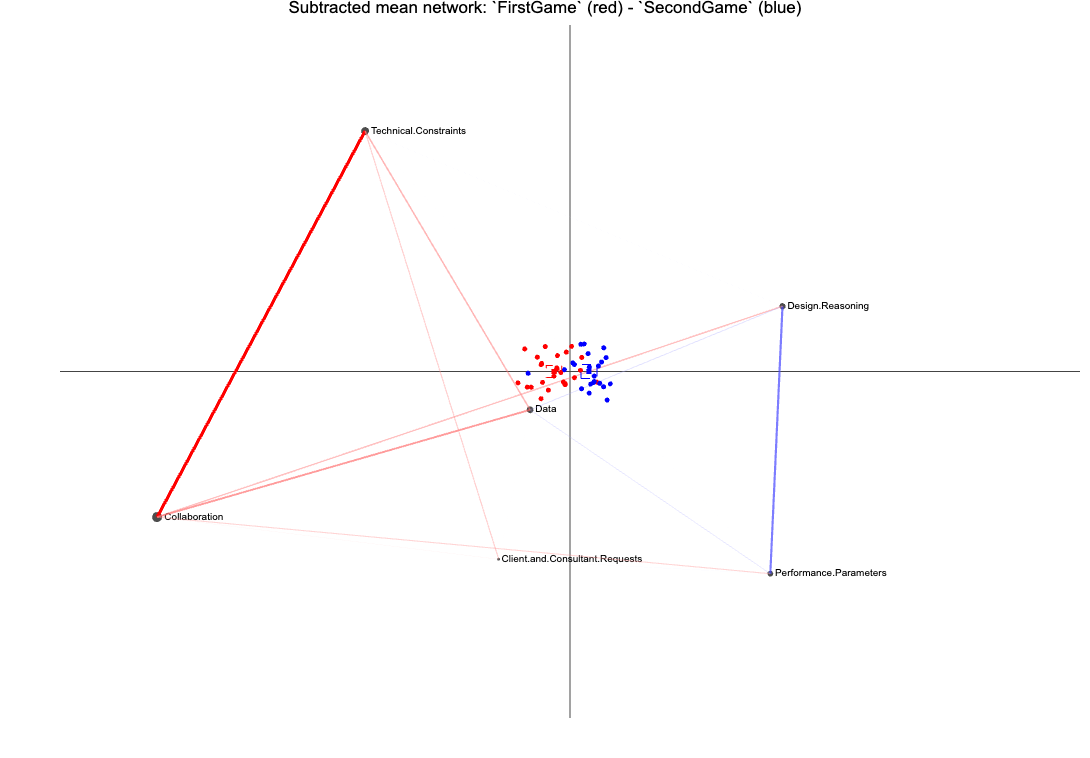
ena.plot(set.ena, title = "Subtracted: `FirstGame` (red) - `SecondGame` (blue)")  |>
  ena.plot.network(network = subtracted.mean * 5, # Optional rescaling of the line weights
                   colors = c("red", "blue"))

Here, the subtracted network shows that on average, students in the FirstGame condition (red) made more connections with Technical.Constraints and Collaboration than students in the SecondGame condition (blue), while students in the SecondGame condition made more connections with Design.Reasoning and Performance.Parameters than students in the FirstGame condition. This is because students with more experience of engineering design practices did not need to spend as much time and effort managing the collaborative process and learning about the basic technical elements of the problem space, and instead spent relatively more time focusing on more complex analysis and design reasoning tasks.

Note

Note: This subtracted network shows no connection between Technical.Constraints and Design.Reasoning, simply because the strength of this connection was similar in both conditions. Thus, subtraction networks should always be visualized along with with the two networks being subtracted.

And instead subtracting to highlight the differences between groups, we could also simply plot all nodes and edges on the same graph to illustrate the most frequent codes and their connections for all participants in the study.

To do so, we simply pipe two calls to ena.plot.network() onto a single base plot like so:

ena.plot(set.ena, title = "All Participants") |>
    ena.plot.network(network = first.game.mean)   |>
    ena.plot.network(network = second.game.mean)

❓Questions

Use the graphs above to answer the following questions and aid in their interpretation:

  1. Overall Density: How does the overall thickness and number of lines differ between the two conditions? What might an increase (or decrease) in network density from FirstGame to SecondGame tell us about how students’ conceptual connections evolved?

    • YOUR RESPONSE HERE
  2. Key Hubs: Which code appears as the strongest “hub” (i.e., connected to more codes)? Did the centrality of that code change between FirstGame and SecondGame? What might that suggest

    • YOUR RESPONSE HERE
  3. Emerging Connections: Are there any code‑pair links that are very faint (or absent) in FirstGame but noticeably stronger in SecondGame? What might this reflect?

    • YOUR RESPONSE HERE
  4. Peripheral Codes: How does the position and edge thickness of the “Collaboration” node change between conditions? What might its relative isolation (or growth) indicate about the role of collaboration in each game?

    • YOUR RESPONSE HERE
  5. Interpretive Meaning: How might you explain the educational significance of a thicker edge versus a thinner edge in these plots, and larger plot points and smaller plot points?

    • YOUR RESPONSE HERE

Plot a mean network and its points

The ENA point or points associated with a network or mean network can also be visualized. Recall from our readings that each individual epistemic network frame can be collapsed to a single point on our graph.

To visualize the points associated with each of the mean networks plotted above, use set$pointsto subset the rows that are in each condition and plot each condition as a different color.

# Subset rotated points for the first condition
first.game.points = as.matrix(set.ena$points$Condition$FirstGame)

# Subset rotated points for the second condition
second.game.points = as.matrix(set.ena$points$Condition$SecondGame)

Then, plot the FirstGame mean network the same as above using ena.plot.network, use |> to pipe in the FirstGame points that we want to include, and plot them using ena.plot.points.

Each point in the space is the ENA point for a given unit. The red and blue squares on the x-axis are the means of the ENA points for each condition, along with the 95% confidence interval on each dimension (you might need to zoom in for better readability)

Since we used a means rotation to construct the ENA model, the resulting space highlights the differences between FirstGame and SecondGame by constructing a rotation that places the means of each condition as close as possible to the x-axis of the space and maximizes the differences between them.

ena.plot(set.ena, title = " points (dots), mean point (square), and confidence interval (box)") |> 
          ena.plot.points(points = first.game.points, colors = c("red")) |> 
          ena.plot.group(point = first.game.points, colors =c("red"), 
                         confidence.interval = "box")

Now let’s overlay the mean graph over these points:

ena.plot(set.ena, title = "FirstGame mean network and its points") |> 
          ena.plot.network(network = first.game.mean, colors = c("red")) |>
          ena.plot.points(points = first.game.points, colors = c("red")) |> 
          ena.plot.group(point = first.game.points, colors =c("red"), 
                         confidence.interval = "box") 

👉 Your Turn ⤵

Now do the same for the SecondGame condition.

# YOUR CODE HERE
ena.plot(set.ena, title = " points (dots), mean point (square), and confidence interval (box)") |> 
          ena.plot.points(points = second.game.points, colors = c("blue")) |> 
          ena.plot.group(point = second.game.points, colors =c("blue"), 
                         confidence.interval = "box")

ena.plot(set.ena, title = "SecondGame mean network and its points") |> 
          ena.plot.network(network = second.game.mean, colors = c("blue")) |>
          ena.plot.points(points = second.game.points, colors = c("blue")) |> 
          ena.plot.group(point = second.game.points, colors =c("blue"), 
                         confidence.interval = "box")

Finally, let’s do the same for subtraction as well:

ena.plot(set.ena, title = "Subtracted mean network: `FirstGame` (red) - `SecondGame` (blue)")  |>
          ena.plot.network(network = subtracted.mean * 5,
          colors = c("red", "blue")) |>
          ena.plot.points(points = first.game.points, colors = c("red")) |> 
          ena.plot.group(point = first.game.points, colors =c("red"), 
                         confidence.interval = "box") |>
          ena.plot.points(points = second.game.points, colors = c("blue")) |> 
          ena.plot.group(point = second.game.points, colors =c("blue"), 
                         confidence.interval = "box")

Note that the majority of the red points (FirstGame) are located on the left side of the space, and the blue points (SecondGame) are mostly located on the right side of the space. This is consistent with the line weights distribution in the mean network: the FirstGame units make relatively more connections with nodes on the left side of the space, while the SecondGame units make relatively more connections with nodes on the right side of the space. The positions of the nodes enable interpretation of the dimensions, and thus interpretation of the locations of the ENA points.

Plot an individual unit network and its point

Plotting the network and ENA point for a single unit uses the same approach. First, subset the line weights and point for a given unit:

unit.A.line.weights = as.matrix(set.ena$line.weights$ENA_UNIT$`FirstGame.steven z`) # subset line weights
unit.A.point = as.matrix(set.ena$points$ENA_UNIT$`FirstGame.steven z`) # subset ENA point

Then, plot the network and point for that unit.

ena.plot(set.ena, title = "Individual network: `FirstGame`.steven z") |> 
          ena.plot.network(network = unit.A.line.weights, colors = c("red")) |>
          ena.plot.points(points = unit.A.point, colors = c("red"))

👉 Your Turn ⤵

Follow the exact same procedure to choose a unit from the other condition to plot and also construct a subtracted plot for those two units.

# YOUR CODE HERE
unit.B.line.weights = as.matrix(set.ena$line.weights$ENA_UNIT$`SecondGame.samuel o`) # subset line weights
unit.B.point = as.matrix(set.ena$points$ENA_UNIT$`SecondGame.samuel o`) # subset ENA point

ena.plot(set.ena, title = "Individual network: `SecondGame`.samuel o") |> 
          ena.plot.network(network = unit.B.line.weights, colors = c("blue")) |>
          ena.plot.points(points = unit.B.point, colors = c("blue"))

To visually analyze the differences between the two individual networks, we can also plot their subtracted network.

ena.plot(set.ena, title = "Subtracted network: `FirstGame`.steven z (red) - `SecondGame`.samuel o (blue)")  |>
          ena.plot.network(network = (unit.A.line.weights - unit.B.line.weights) * 5,
          colors = c("red", "blue")) |>
          ena.plot.points(points = unit.A.point, colors = c("red")) |> 
          ena.plot.points(points = unit.B.point, colors = c("blue"))

In this unit-level subtracted network, Unit A (red) made relatively more connections with codes such as Technical.ConstraintsData, and Collaboration, while Unit B (blue) made relatively more connections with Design.Reasoning and Performance.Parameters.

Plot everything, everywhere, all at once

The helper function ena.plotter enables users to plot points, means, and networks for each condition at the same time. This gives the same results as above more effecient. However, this approach does not enable customization of edge and point colors.

#with helper function
p <-ena.plotter(set.ena,
            points = T,
            mean = T, 
            network = T,
            print.plots = T,
            groupVar = "Condition",
            groups = c("SecondGame","FirstGame"),
            subtractionMultiplier = 5)
$SecondGame

$FirstGame

$`SecondGame-FirstGame`
class(p) <- c("plotly", "enaplot", "html-fill-item-overflow-hidden", "html-fill-item", class(p))

3a. Descriptive Summary of Key Model Outputs

We can also explore descriptive summaries of data stored in the set.ena model by simply extracting the summary data using the handy $ dollar sign operator.

Connection counts

For each unit, in our case individual study participants, ENA creates a cumulative adjacency vector that contains the sums of all unique code co-occurrences for that unit across all stanza windows. These connection counts are the frequencies of unique connections a unit made among all possible code pairs.

To access ENA adjacency vectors, let’s use $ operator to access connection.counts from our set.ena object:

set.ena$connection.counts
                  ENA_UNIT      Condition       UserName CONFIDENCE.Change
            <ena.metadata> <ena.metadata> <ena.metadata>    <ena.metadata>
 1:     FirstGame.steven z      FirstGame       steven z                 1
 2:      FirstGame.akash v      FirstGame        akash v                 2
 3:  FirstGame.alexander b      FirstGame    alexander b                 1
 4:    FirstGame.brandon l      FirstGame      brandon l                 1
 5:  FirstGame.christian x      FirstGame    christian x                 0
 6:     FirstGame.jordan l      FirstGame       jordan l                 2
 7:      FirstGame.arden f      FirstGame        arden f                 1
 8:   FirstGame.margaret n      FirstGame     margaret n                 3
 9:     FirstGame.connor f      FirstGame       connor f                 0
10:      FirstGame.jimmy i      FirstGame        jimmy i                 2
11:      FirstGame.devin c      FirstGame        devin c                 0
12:    FirstGame.tiffany x      FirstGame      tiffany x                 1
13:     FirstGame.amelia n      FirstGame       amelia n                 1
14:       FirstGame.luis t      FirstGame         luis t                 0
15:     FirstGame.amalia x      FirstGame       amalia x                 1
16:     FirstGame.robert z      FirstGame       robert z                 1
17:     FirstGame.joseph k      FirstGame       joseph k                 2
18:      FirstGame.peter h      FirstGame        peter h                 1
19:       FirstGame.carl b      FirstGame         carl b                 1
20:   FirstGame.mitchell h      FirstGame     mitchell h                 1
21:      FirstGame.peter s      FirstGame        peter s                 1
22:     FirstGame.joseph h      FirstGame       joseph h                 2
23:    FirstGame.cameron k      FirstGame      cameron k                 1
24:   FirstGame.fletcher l      FirstGame     fletcher l                 1
25:     FirstGame.amirah u      FirstGame       amirah u                 2
26:      FirstGame.kevin g      FirstGame        kevin g                 1
27:     SecondGame.brent p     SecondGame        brent p                 1
28:     SecondGame.kiana k     SecondGame        kiana k                 1
29:  SecondGame.madeline g     SecondGame     madeline g                 0
30:    SecondGame.justin y     SecondGame       justin y                 1
31:    SecondGame.ruzhen e     SecondGame       ruzhen e                 1
32:   SecondGame.brandon f     SecondGame      brandon f                 1
33:   SecondGame.jackson p     SecondGame      jackson p                 1
34:     SecondGame.shane t     SecondGame        shane t                 1
35:    SecondGame.samuel o     SecondGame       samuel o                 1
36:     SecondGame.casey f     SecondGame        casey f                 1
37:    SecondGame.keegan q     SecondGame       keegan q                 1
38:  SecondGame.nicholas l     SecondGame     nicholas l                 1
39:   SecondGame.cameron i     SecondGame      cameron i                 1
40:   SecondGame.cormick u     SecondGame      cormick u                 0
41:    SecondGame.daniel t     SecondGame       daniel t                 0
42: SecondGame.christina b     SecondGame    christina b                 0
43:     SecondGame.derek v     SecondGame        derek v                 0
44:  SecondGame.nicholas n     SecondGame     nicholas n                 1
45:   SecondGame.abigail z     SecondGame      abigail z                NA
46:   SecondGame.caitlyn y     SecondGame      caitlyn y                 1
47:    SecondGame.nathan d     SecondGame       nathan d                 1
48:      SecondGame.luke u     SecondGame         luke u                 0
                  ENA_UNIT      Condition       UserName CONFIDENCE.Change
    CONFIDENCE.Pre CONFIDENCE.Post       C.Change Data & Technical.Constraints
    <ena.metadata>  <ena.metadata> <ena.metadata>          <ena.co.occurrence>
 1:              7               8     Pos.Change                           22
 2:              6               8     Pos.Change                           47
 3:              5               7     Pos.Change                            9
 4:              5               6     Pos.Change                           98
 5:              4               4     Neg.Change                            6
 6:              6               8     Pos.Change                           24
 7:              5               7     Pos.Change                            8
 8:              4               7     Pos.Change                           15
 9:              6               6     Neg.Change                           20
10:              5               8     Pos.Change                           21
11:              7               7     Pos.Change                            6
12:              6               7     Pos.Change                           21
13:              5               7     Pos.Change                           14
14:              7               7     Pos.Change                           15
15:              5               7     Pos.Change                           23
16:              7               8     Pos.Change                           55
17:              6               8     Pos.Change                           82
18:              4               4     Pos.Change                           25
19:              7               8     Pos.Change                           43
20:              4               4     Pos.Change                           19
21:              4               4     Pos.Change                           12
22:              6               8     Pos.Change                           43
23:              6               7     Pos.Change                           23
24:              6               7     Pos.Change                           16
25:              4               6     Pos.Change                            7
26:              5               6     Pos.Change                           18
27:              5               6     Pos.Change                           12
28:              5               6     Pos.Change                           13
29:              7               7     Pos.Change                           12
30:              5               6     Pos.Change                           24
31:              7               8     Pos.Change                           10
32:              5               6     Pos.Change                           41
33:              6               7     Pos.Change                           20
34:              7               8     Pos.Change                           16
35:              7               8     Pos.Change                            9
36:              7               8     Pos.Change                           15
37:              5               6     Pos.Change                           22
38:              4               4     Pos.Change                           21
39:              6               7     Pos.Change                           31
40:              6               6     Neg.Change                           12
41:              6               6     Neg.Change                           12
42:              4               4     Neg.Change                            9
43:              6               6     Neg.Change                           10
44:              4               4     Pos.Change                           18
45:             NA              NA           #N/A                           10
46:              5               6     Pos.Change                           17
47:              4               4     Pos.Change                           13
48:              7               7     Pos.Change                            6
    CONFIDENCE.Pre CONFIDENCE.Post       C.Change Data & Technical.Constraints
    Data & Performance.Parameters
              <ena.co.occurrence>
 1:                            18
 2:                            34
 3:                             5
 4:                            92
 5:                             5
 6:                            18
 7:                             5
 8:                            12
 9:                            19
10:                            20
11:                             2
12:                            21
13:                             9
14:                            12
15:                            23
16:                            27
17:                            36
18:                            10
19:                            24
20:                             8
21:                             2
22:                            29
23:                            16
24:                            20
25:                             3
26:                            10
27:                             6
28:                             5
29:                            15
30:                            10
31:                            11
32:                            31
33:                            15
34:                            17
35:                            14
36:                            17
37:                            16
38:                            15
39:                            20
40:                            12
41:                            14
42:                            12
43:                             7
44:                            14
45:                            11
46:                             9
47:                            15
48:                             9
    Data & Performance.Parameters
    Technical.Constraints & Performance.Parameters
                               <ena.co.occurrence>
 1:                                             20
 2:                                             42
 3:                                              8
 4:                                             86
 5:                                              6
 6:                                             31
 7:                                              7
 8:                                             12
 9:                                             21
10:                                             22
11:                                              7
12:                                             22
13:                                             11
14:                                             13
15:                                             23
16:                                             30
17:                                             53
18:                                             19
19:                                             29
20:                                             19
21:                                              9
22:                                             37
23:                                             25
24:                                             17
25:                                              8
26:                                             12
27:                                             11
28:                                              9
29:                                             15
30:                                             17
31:                                             13
32:                                             43
33:                                             28
34:                                             18
35:                                             17
36:                                             14
37:                                             19
38:                                             22
39:                                             36
40:                                             18
41:                                              9
42:                                              8
43:                                             12
44:                                             14
45:                                             10
46:                                             18
47:                                             13
48:                                             10
    Technical.Constraints & Performance.Parameters
    Data & Client.and.Consultant.Requests
                      <ena.co.occurrence>
 1:                                     5
 2:                                    10
 3:                                     5
 4:                                    26
 5:                                     2
 6:                                    12
 7:                                     0
 8:                                     4
 9:                                     9
10:                                    10
11:                                     0
12:                                     5
13:                                     2
14:                                     5
15:                                     5
16:                                    10
17:                                    21
18:                                     3
19:                                     6
20:                                     2
21:                                     1
22:                                    14
23:                                     4
24:                                     2
25:                                     4
26:                                     4
27:                                     2
28:                                     6
29:                                     2
30:                                     1
31:                                     6
32:                                    12
33:                                     6
34:                                     8
35:                                     3
36:                                     3
37:                                     2
38:                                     7
39:                                    11
40:                                     3
41:                                     3
42:                                     0
43:                                     5
44:                                     1
45:                                     2
46:                                     2
47:                                     7
48:                                     5
    Data & Client.and.Consultant.Requests
    Technical.Constraints & Client.and.Consultant.Requests
                                       <ena.co.occurrence>
 1:                                                      6
 2:                                                     14
 3:                                                      3
 4:                                                     22
 5:                                                      2
 6:                                                     18
 7:                                                      1
 8:                                                      6
 9:                                                     11
10:                                                     11
11:                                                      2
12:                                                      6
13:                                                      4
14:                                                      6
15:                                                      5
16:                                                     11
17:                                                     26
18:                                                      1
19:                                                      6
20:                                                      3
21:                                                      3
22:                                                     13
23:                                                     11
24:                                                      2
25:                                                      6
26:                                                      5
27:                                                      2
28:                                                      6
29:                                                      1
30:                                                      4
31:                                                      3
32:                                                     15
33:                                                      5
34:                                                      5
35:                                                      3
36:                                                      4
37:                                                      0
38:                                                      7
39:                                                      8
40:                                                      3
41:                                                      0
42:                                                      0
43:                                                      3
44:                                                      0
45:                                                      1
46:                                                      3
47:                                                      6
48:                                                      3
    Technical.Constraints & Client.and.Consultant.Requests
    Performance.Parameters & Client.and.Consultant.Requests
                                        <ena.co.occurrence>
 1:                                                       5
 2:                                                      13
 3:                                                       3
 4:                                                      27
 5:                                                       3
 6:                                                      13
 7:                                                       1
 8:                                                       5
 9:                                                      12
10:                                                      11
11:                                                       0
12:                                                       7
13:                                                       3
14:                                                       5
15:                                                       7
16:                                                       8
17:                                                      16
18:                                                       2
19:                                                       5
20:                                                       1
21:                                                       2
22:                                                      11
23:                                                       8
24:                                                       6
25:                                                       5
26:                                                       3
27:                                                       3
28:                                                       5
29:                                                       5
30:                                                       3
31:                                                       6
32:                                                      14
33:                                                       7
34:                                                      11
35:                                                       7
36:                                                       4
37:                                                       2
38:                                                       7
39:                                                      12
40:                                                       6
41:                                                       2
42:                                                       2
43:                                                       4
44:                                                       1
45:                                                       2
46:                                                       4
47:                                                       6
48:                                                       6
    Performance.Parameters & Client.and.Consultant.Requests
    Data & Design.Reasoning Technical.Constraints & Design.Reasoning
        <ena.co.occurrence>                      <ena.co.occurrence>
 1:                      21                                       26
 2:                      45                                       59
 3:                       5                                        8
 4:                     116                                      110
 5:                       3                                        5
 6:                      25                                       41
 7:                       5                                        8
 8:                      15                                       11
 9:                      17                                       19
10:                      27                                       34
11:                       6                                        9
12:                      21                                       30
13:                      13                                       19
14:                      12                                       13
15:                      26                                       23
16:                      47                                       59
17:                      73                                       88
18:                      24                                       35
19:                      42                                       46
20:                      11                                       25
21:                       8                                       17
22:                      41                                       53
23:                      18                                       33
24:                      27                                       26
25:                       9                                       12
26:                      13                                       21
27:                       9                                       19
28:                      13                                       16
29:                      20                                       13
30:                      23                                       31
31:                      14                                       15
32:                      34                                       59
33:                      24                                       35
34:                      25                                       23
35:                      13                                       18
36:                      17                                       16
37:                      26                                       31
38:                      23                                       32
39:                      28                                       55
40:                      19                                       30
41:                      18                                       11
42:                      10                                       11
43:                      13                                       21
44:                      28                                       36
45:                      12                                       11
46:                      12                                       17
47:                      14                                       16
48:                       9                                        8
    Data & Design.Reasoning Technical.Constraints & Design.Reasoning
    Performance.Parameters & Design.Reasoning
                          <ena.co.occurrence>
 1:                                        19
 2:                                        38
 3:                                         5
 4:                                        98
 5:                                         5
 6:                                        32
 7:                                         3
 8:                                        10
 9:                                        18
10:                                        26
11:                                         7
12:                                        18
13:                                        14
14:                                         9
15:                                        23
16:                                        27
17:                                        44
18:                                        19
19:                                        33
20:                                         7
21:                                         9
22:                                        45
23:                                        26
24:                                        32
25:                                         9
26:                                        11
27:                                         8
28:                                         8
29:                                        22
30:                                        17
31:                                        21
32:                                        37
33:                                        31
34:                                        24
35:                                        22
36:                                        21
37:                                        31
38:                                        21
39:                                        30
40:                                        23
41:                                        12
42:                                        10
43:                                        16
44:                                        23
45:                                        14
46:                                        13
47:                                        14
48:                                        12
    Performance.Parameters & Design.Reasoning
    Client.and.Consultant.Requests & Design.Reasoning Data & Collaboration
                                  <ena.co.occurrence>  <ena.co.occurrence>
 1:                                                 6                    7
 2:                                                 9                   12
 3:                                                 2                    4
 4:                                                26                   30
 5:                                                 1                    1
 6:                                                22                   10
 7:                                                 0                    3
 8:                                                 5                    8
 9:                                                12                    9
10:                                                14                   10
11:                                                 1                    1
12:                                                10                    9
13:                                                 6                    3
14:                                                 5                    9
15:                                                 7                    8
16:                                                13                   11
17:                                                22                   28
18:                                                 5                    6
19:                                                 7                    6
20:                                                 1                    5
21:                                                 3                    2
22:                                                17                    4
23:                                                12                    7
24:                                                10                    8
25:                                                 7                    3
26:                                                 7                    5
27:                                                 3                    1
28:                                                 4                    6
29:                                                 5                    4
30:                                                 4                    1
31:                                                 6                    2
32:                                                16                   12
33:                                                10                    0
34:                                                11                    4
35:                                                 8                    0
36:                                                 6                    1
37:                                                 1                    1
38:                                                 6                    5
39:                                                10                    0
40:                                                 7                    1
41:                                                 4                    3
42:                                                 2                    3
43:                                                10                    1
44:                                                 4                    2
45:                                                 2                    0
46:                                                 3                    3
47:                                                 6                    1
48:                                                 6                    1
    Client.and.Consultant.Requests & Design.Reasoning Data & Collaboration
    Technical.Constraints & Collaboration
                      <ena.co.occurrence>
 1:                                     9
 2:                                    21
 3:                                     6
 4:                                    29
 5:                                     2
 6:                                    30
 7:                                     3
 8:                                     4
 9:                                    12
10:                                    10
11:                                     3
12:                                    11
13:                                     7
14:                                    10
15:                                    10
16:                                    13
17:                                    32
18:                                     5
19:                                     4
20:                                    11
21:                                     6
22:                                     8
23:                                    16
24:                                     4
25:                                     7
26:                                     9
27:                                     0
28:                                     7
29:                                     4
30:                                     2
31:                                     2
32:                                    10
33:                                     2
34:                                     6
35:                                     2
36:                                     2
37:                                     2
38:                                     6
39:                                     4
40:                                     2
41:                                     1
42:                                     0
43:                                     3
44:                                     0
45:                                     1
46:                                     2
47:                                     1
48:                                     0
    Technical.Constraints & Collaboration
    Performance.Parameters & Collaboration
                       <ena.co.occurrence>
 1:                                      7
 2:                                     11
 3:                                      4
 4:                                     15
 5:                                      2
 6:                                     14
 7:                                      2
 8:                                      5
 9:                                      9
10:                                      7
11:                                      1
12:                                      6
13:                                      3
14:                                      5
15:                                      5
16:                                      8
17:                                     14
18:                                      3
19:                                      2
20:                                      7
21:                                      2
22:                                     10
23:                                      7
24:                                      5
25:                                      1
26:                                      6
27:                                      1
28:                                      5
29:                                      5
30:                                      1
31:                                      3
32:                                      7
33:                                      3
34:                                      5
35:                                      1
36:                                      2
37:                                      1
38:                                      4
39:                                      0
40:                                      3
41:                                      2
42:                                      3
43:                                      1
44:                                      2
45:                                      4
46:                                      3
47:                                      1
48:                                      1
    Performance.Parameters & Collaboration
    Client.and.Consultant.Requests & Collaboration
                               <ena.co.occurrence>
 1:                                              1
 2:                                              2
 3:                                              0
 4:                                              2
 5:                                              0
 6:                                             10
 7:                                              1
 8:                                              3
 9:                                              5
10:                                              4
11:                                              0
12:                                              4
13:                                              4
14:                                              2
15:                                              3
16:                                              2
17:                                              7
18:                                              0
19:                                              0
20:                                              1
21:                                              1
22:                                              3
23:                                              0
24:                                              3
25:                                              3
26:                                              0
27:                                              0
28:                                              3
29:                                              2
30:                                              0
31:                                              0
32:                                             11
33:                                              2
34:                                              4
35:                                              0
36:                                              0
37:                                              1
38:                                              2
39:                                              1
40:                                              1
41:                                              1
42:                                              0
43:                                              1
44:                                              1
45:                                              0
46:                                              1
47:                                              0
48:                                              1
    Client.and.Consultant.Requests & Collaboration
    Design.Reasoning & Collaboration
                 <ena.co.occurrence>
 1:                                6
 2:                               19
 3:                                5
 4:                               38
 5:                                0
 6:                               28
 7:                                2
 8:                                6
 9:                               13
10:                               13
11:                                2
12:                               11
13:                                8
14:                                5
15:                               11
16:                               10
17:                               30
18:                                6
19:                                8
20:                               10
21:                                5
22:                               11
23:                                6
24:                                6
25:                                6
26:                                5
27:                                2
28:                               10
29:                                9
30:                                1
31:                                2
32:                               20
33:                                6
34:                               10
35:                                2
36:                                3
37:                                2
38:                                5
39:                                4
40:                                3
41:                                5
42:                                2
43:                                4
44:                                2
45:                                6
46:                                3
47:                                1
48:                                1
    Design.Reasoning & Collaboration

This data table shows summaries of connection counts for the 48 units (i.e., the 48 study participants and whether this was their first or second game) that are stored in the ENA model. Each term, or column in this table, represents a unique co-occurrence of codes.

In the first row, we can see that among steven z’s conversations, the codes Data and Technical.Constraints occurred together 22 times, whereas for brandon l’s conversations, Data and Technical.Constraints occurred together 98 times!

Tip

The $ Operator. In R, the $ operator is simply a shortcut for “extract the element named … from this object.” So in set.ena$connection.counts, for example, we’re pulling out the component named connection.counts from the set.ena object.

In general, whenever you have a list, data frame, or environment, you can write object$elementName to retrieve the item (e.g., a column, sub‑list, etc.) whose name exactly matches elementName.

👉 Your Turn ⤵

We can also take these data summaries a step further by using the skim() function introduced in previous units to get summary statistics for all code pairs collectively.

Use the code chunk below to load the {skimr} library and skim() the set.ena$connection.counts to get a descriptive summary of connection counts for each participant:

#YOUR CODE HERE

library(skimr)

set.ena$connection.counts |>
  skimr::skim()
Data summary
Name set.ena$connection.counts
Number of rows 48
Number of columns 22
Key NULL
_______________________
Column type frequency:
character 7
numeric 15
________________________
Group variables None

Variable type: character

skim_variable n_missing complete_rate min max empty n_unique whitespace
ENA_UNIT 0 1.00 16 22 0 48 0
Condition 0 1.00 9 10 0 2 0
UserName 0 1.00 6 11 0 48 0
CONFIDENCE.Change 1 0.98 1 1 0 4 0
CONFIDENCE.Pre 1 0.98 1 1 0 4 0
CONFIDENCE.Post 1 0.98 1 1 0 4 0
C.Change 0 1.00 4 10 0 3 0

Variable type: numeric

skim_variable n_missing complete_rate mean sd p0 p25 p50 p75 p100 hist
Data & Technical.Constraints 0 1 21.77 18.21 6 12.00 16.5 23.00 98 ▇▁▁▁▁
Data & Performance.Parameters 0 1 16.15 13.76 2 9.00 14.0 19.25 92 ▇▂▁▁▁
Technical.Constraints & Performance.Parameters 0 1 20.06 14.28 6 11.00 17.0 22.25 86 ▇▂▁▁▁
Data & Client.and.Consultant.Requests 0 1 5.58 5.13 0 2.00 4.5 7.00 26 ▇▃▁▁▁
Technical.Constraints & Client.and.Consultant.Requests 0 1 5.96 5.66 0 2.75 4.5 6.25 26 ▇▃▂▁▁
Performance.Parameters & Client.and.Consultant.Requests 0 1 6.27 4.92 0 3.00 5.0 7.25 27 ▇▃▃▁▁
Data & Design.Reasoning 0 1 22.38 18.91 3 12.00 18.0 26.00 116 ▇▂▁▁▁
Technical.Constraints & Design.Reasoning 0 1 28.21 20.95 5 14.50 22.0 34.25 110 ▇▃▂▁▁
Performance.Parameters & Design.Reasoning 0 1 21.19 15.39 3 10.75 19.0 26.25 98 ▇▃▁▁▁
Client.and.Consultant.Requests & Design.Reasoning 0 1 7.58 5.75 0 4.00 6.0 10.00 26 ▇▇▂▁▁
Data & Collaboration 0 1 5.44 6.07 0 1.00 4.0 8.00 30 ▇▃▁▁▁
Technical.Constraints & Collaboration 0 1 7.10 7.55 0 2.00 4.5 10.00 32 ▇▃▁▁▁
Performance.Parameters & Collaboration 0 1 4.56 3.64 0 2.00 3.5 6.25 15 ▇▃▂▁▁
Client.and.Consultant.Requests & Collaboration 0 1 1.94 2.41 0 0.00 1.0 3.00 11 ▇▂▁▁▁
Design.Reasoning & Collaboration 0 1 7.77 7.76 0 2.75 6.0 10.00 38 ▇▃▁▁▁

❓Questions

Take a closer look at the table output above and answer the following questions:

  1. Which code pair has the highest mean co‑occurrence count? What is that mean value?
    • YOUR RESPONSE HERE
  2. Which code pair has the lowest mean co‑occurrence count?
    • YOUR RESPONSE HERE
  3. Which code pair reaches the highest maximum value (p100)? How many times does that relationship appear in its strongest instance?
    • YOUR RESPONSE HERE
  4. Name all code pairs whose minimum (p0) value is zero. What does a zero minimum indicate about those relationships?
    • YOUR RESPONSE HERE

Line weights

These raw connection counts can also be rerpresented as line weights, or normalized relative frequencies (i.e., decimal values between 0 and 1) of code co-occurrence for each unit by dividing each code‑pair count by the total number of connections for that unit or individuals.

Why normalize? Because some participants might talk a lot (producing high raw counts) while others talk less. By converting counts into proportions, we compare patterns of emphasis (which code pairs are relatively important) instead of comparing raw activity levels.

👉 Your Turn ⤵

Similar to how we extracted the conneciton counts data from our set.ena object above, use the $ operator To access the normalized adjacency vectors, use set.ena$line.weights.

set.ena$line.weights
                  ENA_UNIT      Condition       UserName CONFIDENCE.Change
            <ena.metadata> <ena.metadata> <ena.metadata>    <ena.metadata>
 1:     FirstGame.steven z      FirstGame       steven z                 1
 2:      FirstGame.akash v      FirstGame        akash v                 2
 3:  FirstGame.alexander b      FirstGame    alexander b                 1
 4:    FirstGame.brandon l      FirstGame      brandon l                 1
 5:  FirstGame.christian x      FirstGame    christian x                 0
 6:     FirstGame.jordan l      FirstGame       jordan l                 2
 7:      FirstGame.arden f      FirstGame        arden f                 1
 8:   FirstGame.margaret n      FirstGame     margaret n                 3
 9:     FirstGame.connor f      FirstGame       connor f                 0
10:      FirstGame.jimmy i      FirstGame        jimmy i                 2
11:      FirstGame.devin c      FirstGame        devin c                 0
12:    FirstGame.tiffany x      FirstGame      tiffany x                 1
13:     FirstGame.amelia n      FirstGame       amelia n                 1
14:       FirstGame.luis t      FirstGame         luis t                 0
15:     FirstGame.amalia x      FirstGame       amalia x                 1
16:     FirstGame.robert z      FirstGame       robert z                 1
17:     FirstGame.joseph k      FirstGame       joseph k                 2
18:      FirstGame.peter h      FirstGame        peter h                 1
19:       FirstGame.carl b      FirstGame         carl b                 1
20:   FirstGame.mitchell h      FirstGame     mitchell h                 1
21:      FirstGame.peter s      FirstGame        peter s                 1
22:     FirstGame.joseph h      FirstGame       joseph h                 2
23:    FirstGame.cameron k      FirstGame      cameron k                 1
24:   FirstGame.fletcher l      FirstGame     fletcher l                 1
25:     FirstGame.amirah u      FirstGame       amirah u                 2
26:      FirstGame.kevin g      FirstGame        kevin g                 1
27:     SecondGame.brent p     SecondGame        brent p                 1
28:     SecondGame.kiana k     SecondGame        kiana k                 1
29:  SecondGame.madeline g     SecondGame     madeline g                 0
30:    SecondGame.justin y     SecondGame       justin y                 1
31:    SecondGame.ruzhen e     SecondGame       ruzhen e                 1
32:   SecondGame.brandon f     SecondGame      brandon f                 1
33:   SecondGame.jackson p     SecondGame      jackson p                 1
34:     SecondGame.shane t     SecondGame        shane t                 1
35:    SecondGame.samuel o     SecondGame       samuel o                 1
36:     SecondGame.casey f     SecondGame        casey f                 1
37:    SecondGame.keegan q     SecondGame       keegan q                 1
38:  SecondGame.nicholas l     SecondGame     nicholas l                 1
39:   SecondGame.cameron i     SecondGame      cameron i                 1
40:   SecondGame.cormick u     SecondGame      cormick u                 0
41:    SecondGame.daniel t     SecondGame       daniel t                 0
42: SecondGame.christina b     SecondGame    christina b                 0
43:     SecondGame.derek v     SecondGame        derek v                 0
44:  SecondGame.nicholas n     SecondGame     nicholas n                 1
45:   SecondGame.abigail z     SecondGame      abigail z                NA
46:   SecondGame.caitlyn y     SecondGame      caitlyn y                 1
47:    SecondGame.nathan d     SecondGame       nathan d                 1
48:      SecondGame.luke u     SecondGame         luke u                 0
                  ENA_UNIT      Condition       UserName CONFIDENCE.Change
    CONFIDENCE.Pre CONFIDENCE.Post       C.Change Data & Technical.Constraints
    <ena.metadata>  <ena.metadata> <ena.metadata>          <ena.co.occurrence>
 1:              7               8     Pos.Change                    0.4000661
 2:              6               8     Pos.Change                    0.4016067
 3:              5               7     Pos.Change                    0.4370786
 4:              5               6     Pos.Change                    0.3797337
 5:              4               4     Neg.Change                    0.4435328
 6:              6               8     Pos.Change                    0.2619863
 7:              5               7     Pos.Change                    0.4914361
 8:              4               7     Pos.Change                    0.4310416
 9:              6               6     Neg.Change                    0.3554467
10:              5               8     Pos.Change                    0.3012940
11:              7               7     Pos.Change                    0.3618136
12:              6               7     Pos.Change                    0.3492248
13:              5               7     Pos.Change                    0.3830230
14:              7               7     Pos.Change                    0.4195907
15:              5               7     Pos.Change                    0.3736998
16:              7               8     Pos.Change                    0.5023931
17:              6               8     Pos.Change                    0.4683956
18:              4               4     Pos.Change                    0.4291885
19:              7               8     Pos.Change                    0.4663731
20:              4               4     Pos.Change                    0.4368105
21:              4               4     Pos.Change                    0.4364358
22:              6               8     Pos.Change                    0.3982335
23:              6               7     Pos.Change                    0.3534699
24:              6               7     Pos.Change                    0.2641833
25:              4               6     Pos.Change                    0.2728884
26:              5               6     Pos.Change                    0.4550041
27:              5               6     Pos.Change                    0.4142860
28:              5               6     Pos.Change                    0.3926794
29:              7               7     Pos.Change                    0.2794479
30:              5               6     Pos.Change                    0.4541254
31:              7               8     Pos.Change                    0.2682209
32:              5               6     Pos.Change                    0.3722354
33:              6               7     Pos.Change                    0.3003531
34:              7               8     Pos.Change                    0.2863083
35:              7               8     Pos.Change                    0.2193817
36:              7               8     Pos.Change                    0.3544406
37:              5               6     Pos.Change                    0.3607527
38:              4               4     Pos.Change                    0.3584119
39:              6               7     Pos.Change                    0.3503776
40:              6               6     Neg.Change                    0.2386200
41:              6               6     Neg.Change                    0.3653175
42:              4               4     Neg.Change                    0.3557562
43:              6               6     Neg.Change                    0.2734855
44:              4               4     Pos.Change                    0.3107145
45:             NA              NA           #N/A                    0.3434014
46:              5               6     Pos.Change                    0.4599637
47:              4               4     Pos.Change                    0.3509670
48:              7               7     Pos.Change                    0.2417469
    CONFIDENCE.Pre CONFIDENCE.Post       C.Change Data & Technical.Constraints
    Data & Performance.Parameters
              <ena.co.occurrence>
 1:                     0.3273268
 2:                     0.2905240
 3:                     0.2428215
 4:                     0.3564847
 5:                     0.3696106
 6:                     0.1964897
 7:                     0.3071476
 8:                     0.3448333
 9:                     0.3376744
10:                     0.2869467
11:                     0.1206045
12:                     0.3492248
13:                     0.2462290
14:                     0.3356725
15:                     0.3736998
16:                     0.2466293
17:                     0.2056371
18:                     0.1716754
19:                     0.2603012
20:                     0.1839202
21:                     0.0727393
22:                     0.2685761
23:                     0.2458921
24:                     0.3302291
25:                     0.1169522
26:                     0.2527801
27:                     0.2071430
28:                     0.1510305
29:                     0.3493098
30:                     0.1892189
31:                     0.2950430
32:                     0.2814463
33:                     0.2252648
34:                     0.3042026
35:                     0.3412605
36:                     0.4016993
37:                     0.2623656
38:                     0.2560085
39:                     0.2260500
40:                     0.2386200
41:                     0.4262038
42:                     0.4743416
43:                     0.1914398
44:                     0.2416668
45:                     0.3777416
46:                     0.2435102
47:                     0.4049619
48:                     0.3626203
    Data & Performance.Parameters
    Technical.Constraints & Performance.Parameters
                               <ena.co.occurrence>
 1:                                      0.3636965
 2:                                      0.3588826
 3:                                      0.3885143
 4:                                      0.3332357
 5:                                      0.4435328
 6:                                      0.3383989
 7:                                      0.4300066
 8:                                      0.3448333
 9:                                      0.3732191
10:                                      0.3156414
11:                                      0.4221159
12:                                      0.3658546
13:                                      0.3009466
14:                                      0.3636453
15:                                      0.3736998
16:                                      0.2740326
17:                                      0.3027435
18:                                      0.3261833
19:                                      0.3145307
20:                                      0.4368105
21:                                      0.3273268
22:                                      0.3426660
23:                                      0.3842064
24:                                      0.2806947
25:                                      0.3118725
26:                                      0.3033361
27:                                      0.3797622
28:                                      0.2718549
29:                                      0.3493098
30:                                      0.3216721
31:                                      0.3486872
32:                                      0.3903932
33:                                      0.4204944
34:                                      0.3220969
35:                                      0.4143877
36:                                      0.3308112
37:                                      0.3115592
38:                                      0.3754791
39:                                      0.4068901
40:                                      0.3579300
41:                                      0.2739882
42:                                      0.3162278
43:                                      0.3281826
44:                                      0.2416668
45:                                      0.3434014
46:                                      0.4870204
47:                                      0.3509670
48:                                      0.4029115
    Technical.Constraints & Performance.Parameters
    Data & Client.and.Consultant.Requests
                      <ena.co.occurrence>
 1:                            0.09092412
 2:                            0.08544824
 3:                            0.24282147
 4:                            0.10074568
 5:                            0.14784425
 6:                            0.13099313
 7:                            0.00000000
 8:                            0.11494443
 9:                            0.15995103
10:                            0.14347335
11:                            0.00000000
12:                            0.08314876
13:                            0.05471757
14:                            0.13986356
15:                            0.08123908
16:                            0.09134420
17:                            0.11995496
18:                            0.05150262
19:                            0.06507531
20:                            0.04598005
21:                            0.03636965
22:                            0.12965742
23:                            0.06147302
24:                            0.03302291
25:                            0.15593624
26:                            0.10111203
27:                            0.06904767
28:                            0.18123663
29:                            0.04657464
30:                            0.01892189
31:                            0.16093253
32:                            0.10894694
33:                            0.09010594
34:                            0.14315417
35:                            0.07312724
36:                            0.07088812
37:                            0.03279570
38:                            0.11947063
39:                            0.12432752
40:                            0.05965500
41:                            0.09132938
42:                            0.00000000
43:                            0.13674275
44:                            0.01726192
45:                            0.06868028
46:                            0.05411338
47:                            0.18898224
48:                            0.20145574
    Data & Client.and.Consultant.Requests
    Technical.Constraints & Client.and.Consultant.Requests
                                       <ena.co.occurrence>
 1:                                             0.10910895
 2:                                             0.11962754
 3:                                             0.14569288
 4:                                             0.08524635
 5:                                             0.14784425
 6:                                             0.19648969
 7:                                             0.06142951
 8:                                             0.17241664
 9:                                             0.19549571
10:                                             0.15782069
11:                                             0.12060454
12:                                             0.09977852
13:                                             0.10943513
14:                                             0.16783627
15:                                             0.08123908
16:                                             0.10047862
17:                                             0.14851567
18:                                             0.01716754
19:                                             0.06507531
20:                                             0.06897007
21:                                             0.10910895
22:                                             0.12039618
23:                                             0.16905081
24:                                             0.03302291
25:                                             0.23390435
26:                                             0.12639003
27:                                             0.06904767
28:                                             0.18123663
29:                                             0.02328732
30:                                             0.07568756
31:                                             0.08046627
32:                                             0.13618368
33:                                             0.07508828
34:                                             0.08947135
35:                                             0.07312724
36:                                             0.09451749
37:                                             0.00000000
38:                                             0.11947063
39:                                             0.09042002
40:                                             0.05965500
41:                                             0.00000000
42:                                             0.00000000
43:                                             0.08204565
44:                                             0.00000000
45:                                             0.03434014
46:                                             0.08117007
47:                                             0.16198477
48:                                             0.12087344
    Technical.Constraints & Client.and.Consultant.Requests
    Performance.Parameters & Client.and.Consultant.Requests
                                        <ena.co.occurrence>
 1:                                              0.09092412
 2:                                              0.11108271
 3:                                              0.14569288
 4:                                              0.10462052
 5:                                              0.22176638
 6:                                              0.14190922
 7:                                              0.06142951
 8:                                              0.14368053
 9:                                              0.21326805
10:                                              0.15782069
11:                                              0.00000000
12:                                              0.11640827
13:                                              0.08207635
14:                                              0.13986356
15:                                              0.11373472
16:                                              0.07307536
17:                                              0.09139426
18:                                              0.03433508
19:                                              0.05422942
20:                                              0.02299002
21:                                              0.07273930
22:                                              0.10187369
23:                                              0.12294604
24:                                              0.09906873
25:                                              0.19492029
26:                                              0.07583402
27:                                              0.10357150
28:                                              0.15103052
29:                                              0.11643661
30:                                              0.05676567
31:                                              0.16093253
32:                                              0.12710477
33:                                              0.10512359
34:                                              0.19683698
35:                                              0.17063023
36:                                              0.09451749
37:                                              0.03279570
38:                                              0.11947063
39:                                              0.13563002
40:                                              0.11931000
41:                                              0.06088626
42:                                              0.07905694
43:                                              0.10939420
44:                                              0.01726192
45:                                              0.06868028
46:                                              0.10822676
47:                                              0.16198477
48:                                              0.24174689
    Performance.Parameters & Client.and.Consultant.Requests
    Data & Design.Reasoning Technical.Constraints & Design.Reasoning
        <ena.co.occurrence>                      <ena.co.occurrence>
 1:               0.3818813                                0.4728054
 2:               0.3845171                                0.5041446
 3:               0.2428215                                0.3885143
 4:               0.4494807                                0.4262317
 5:               0.2217664                                0.3696106
 6:               0.2729023                                0.4475598
 7:               0.3071476                                0.4914361
 8:               0.4310416                                0.3160972
 9:               0.3021297                                0.3376744
10:               0.3873781                                0.4878094
11:               0.3618136                                0.5427204
12:               0.3492248                                0.4988926
13:               0.3556642                                0.5198169
14:               0.3356725                                0.3636453
15:               0.4224432                                0.3736998
16:               0.4293177                                0.5389308
17:               0.4169863                                0.5026684
18:               0.4120210                                0.6008639
19:               0.4555272                                0.4989107
20:               0.2528903                                0.5747506
21:               0.2909572                                0.6182840
22:               0.3797110                                0.4908460
23:               0.2766286                                0.5071524
24:               0.4458093                                0.4292978
25:               0.3508565                                0.4678087
26:               0.3286141                                0.5308381
27:               0.3107145                                0.6559528
28:               0.3926794                                0.4832977
29:               0.4657464                                0.3027352
30:               0.4352035                                0.5865786
31:               0.3755092                                0.4023313
32:               0.3086830                                0.5356558
33:               0.3604237                                0.5256180
34:               0.4473568                                0.4115682
35:               0.3168847                                0.4387635
36:               0.4016993                                0.3780700
37:               0.4263441                                0.5083334
38:               0.3925463                                0.5461514
39:               0.3164701                                0.6216376
40:               0.3778150                                0.5965500
41:               0.5479763                                0.3348744
42:               0.3952847                                0.4348132
43:               0.3555311                                0.5743195
44:               0.4833337                                0.6214290
45:               0.4120817                                0.3777416
46:               0.3246803                                0.4599637
47:               0.3779645                                0.4319594
48:               0.3626203                                0.3223292
    Data & Design.Reasoning Technical.Constraints & Design.Reasoning
    Performance.Parameters & Design.Reasoning
                          <ena.co.occurrence>
 1:                                 0.3455117
 2:                                 0.3247033
 3:                                 0.2428215
 4:                                 0.3797337
 5:                                 0.3696106
 6:                                 0.3493150
 7:                                 0.1842885
 8:                                 0.2873611
 9:                                 0.3199021
10:                                 0.3730307
11:                                 0.4221159
12:                                 0.2993355
13:                                 0.3830230
14:                                 0.2517544
15:                                 0.3736998
16:                                 0.2466293
17:                                 0.2513342
18:                                 0.3261833
19:                                 0.3579142
20:                                 0.1609302
21:                                 0.3273268
22:                                 0.4167560
23:                                 0.3995746
24:                                 0.5283665
25:                                 0.3508565
26:                                 0.2780581
27:                                 0.2761907
28:                                 0.2416488
29:                                 0.5123211
30:                                 0.3216721
31:                                 0.5632639
32:                                 0.3359197
33:                                 0.4655473
34:                                 0.4294625
35:                                 0.5362664
36:                                 0.4962168
37:                                 0.5083334
38:                                 0.3584119
39:                                 0.3390751
40:                                 0.4573550
41:                                 0.3653175
42:                                 0.3952847
43:                                 0.4375768
44:                                 0.3970241
45:                                 0.4807620
46:                                 0.3517370
47:                                 0.3779645
48:                                 0.4834938
    Performance.Parameters & Design.Reasoning
    Client.and.Consultant.Requests & Design.Reasoning Data & Collaboration
                                  <ena.co.occurrence>  <ena.co.occurrence>
 1:                                        0.10910895           0.12729377
 2:                                        0.07690342           0.10253789
 3:                                        0.09712859           0.19425717
 4:                                        0.10074568           0.11624502
 5:                                        0.07392213           0.07392213
 6:                                        0.24015407           0.10916094
 7:                                        0.00000000           0.18428854
 8:                                        0.14368053           0.22988885
 9:                                        0.21326805           0.15995103
10:                                        0.20086269           0.14347335
11:                                        0.06030227           0.06030227
12:                                        0.16629753           0.14966777
13:                                        0.16415270           0.08207635
14:                                        0.13986356           0.25175441
15:                                        0.11373472           0.12998253
16:                                        0.11874746           0.10047862
17:                                        0.12566711           0.15993995
18:                                        0.08583770           0.10300524
19:                                        0.07592119           0.06507531
20:                                        0.02299002           0.11495012
21:                                        0.10910895           0.07273930
22:                                        0.15744116           0.03704498
23:                                        0.18441907           0.10757779
24:                                        0.16511455           0.13209164
25:                                        0.27288841           0.11695218
26:                                        0.17694605           0.12639003
27:                                        0.10357150           0.03452383
28:                                        0.12082442           0.18123663
29:                                        0.11643661           0.09314929
30:                                        0.07568756           0.01892189
31:                                        0.16093253           0.05364418
32:                                        0.14526259           0.10894694
33:                                        0.15017656           0.00000000
34:                                        0.19683698           0.07157708
35:                                        0.19500598           0.00000000
36:                                        0.14177624           0.02362937
37:                                        0.01639785           0.01639785
38:                                        0.10240339           0.08533616
39:                                        0.11302502           0.00000000
40:                                        0.13919500           0.01988500
41:                                        0.12177251           0.09132938
42:                                        0.07905694           0.11858541
43:                                        0.27348549           0.02734855
44:                                        0.06904767           0.03452383
45:                                        0.06868028           0.00000000
46:                                        0.08117007           0.08117007
47:                                        0.16198477           0.02699746
48:                                        0.24174689           0.04029115
    Client.and.Consultant.Requests & Design.Reasoning Data & Collaboration
    Technical.Constraints & Collaboration
                      <ena.co.occurrence>
 1:                            0.16366342
 2:                            0.17944131
 3:                            0.29138576
 4:                            0.11237019
 5:                            0.14784425
 6:                            0.32748282
 7:                            0.18428854
 8:                            0.11494443
 9:                            0.21326805
10:                            0.14347335
11:                            0.18090681
12:                            0.18292728
13:                            0.19151148
14:                            0.27972712
15:                            0.16247817
16:                            0.11874746
17:                            0.18278852
18:                            0.08583770
19:                            0.04338354
20:                            0.25289027
21:                            0.21821789
22:                            0.07408996
23:                            0.24589209
24:                            0.06604582
25:                            0.27288841
26:                            0.22750206
27:                            0.00000000
28:                            0.21144273
29:                            0.09314929
30:                            0.03784378
31:                            0.05364418
32:                            0.09078912
33:                            0.03003531
34:                            0.10736563
35:                            0.04875149
36:                            0.04725875
37:                            0.03279570
38:                            0.10240339
39:                            0.04521001
40:                            0.03977000
41:                            0.03044313
42:                            0.00000000
43:                            0.08204565
44:                            0.00000000
45:                            0.03434014
46:                            0.05411338
47:                            0.02699746
48:                            0.00000000
    Technical.Constraints & Collaboration
    Performance.Parameters & Collaboration
                       <ena.co.occurrence>
 1:                             0.12729377
 2:                             0.09399306
 3:                             0.19425717
 4:                             0.05812251
 5:                             0.14784425
 6:                             0.15282531
 7:                             0.12285902
 8:                             0.14368053
 9:                             0.15995103
10:                             0.10043135
11:                             0.06030227
12:                             0.09977852
13:                             0.08207635
14:                             0.13986356
15:                             0.08123908
16:                             0.07307536
17:                             0.07996998
18:                             0.05150262
19:                             0.02169177
20:                             0.16093017
21:                             0.07273930
22:                             0.09261244
23:                             0.10757779
24:                             0.08255727
25:                             0.03898406
26:                             0.15166804
27:                             0.03452383
28:                             0.15103052
29:                             0.11643661
30:                             0.01892189
31:                             0.08046627
32:                             0.06355238
33:                             0.04505297
34:                             0.08947135
35:                             0.02437575
36:                             0.04725875
37:                             0.01639785
38:                             0.06826893
39:                             0.00000000
40:                             0.05965500
41:                             0.06088626
42:                             0.11858541
43:                             0.02734855
44:                             0.03452383
45:                             0.13736056
46:                             0.08117007
47:                             0.02699746
48:                             0.04029115
    Performance.Parameters & Collaboration
    Client.and.Consultant.Requests & Collaboration
                               <ena.co.occurrence>
 1:                                    0.018184824
 2:                                    0.017089648
 3:                                    0.000000000
 4:                                    0.007749668
 5:                                    0.000000000
 6:                                    0.109160939
 7:                                    0.061429512
 8:                                    0.086208320
 9:                                    0.088861686
10:                                    0.057389341
11:                                    0.000000000
12:                                    0.066519011
13:                                    0.109435131
14:                                    0.055945424
15:                                    0.048743451
16:                                    0.018268840
17:                                    0.039984988
18:                                    0.000000000
19:                                    0.000000000
20:                                    0.022990024
21:                                    0.036369648
22:                                    0.027783733
23:                                    0.000000000
24:                                    0.049534364
25:                                    0.116952176
26:                                    0.000000000
27:                                    0.000000000
28:                                    0.090618314
29:                                    0.046574643
30:                                    0.000000000
31:                                    0.000000000
32:                                    0.099868030
33:                                    0.030035312
34:                                    0.071577084
35:                                    0.000000000
36:                                    0.000000000
37:                                    0.016397850
38:                                    0.034134464
39:                                    0.011302502
40:                                    0.019885000
41:                                    0.030443128
42:                                    0.000000000
43:                                    0.027348549
44:                                    0.017261917
45:                                    0.000000000
46:                                    0.027056689
47:                                    0.000000000
48:                                    0.040291148
    Client.and.Consultant.Requests & Collaboration
    Design.Reasoning & Collaboration
                 <ena.co.occurrence>
 1:                       0.10910895
 2:                       0.16235166
 3:                       0.24282147
 4:                       0.14724369
 5:                       0.00000000
 6:                       0.30565063
 7:                       0.12285902
 8:                       0.17241664
 9:                       0.23104038
10:                       0.18651536
11:                       0.12060454
12:                       0.18292728
13:                       0.21887026
14:                       0.13986356
15:                       0.17872599
16:                       0.09134420
17:                       0.17136423
18:                       0.10300524
19:                       0.08676708
20:                       0.22990024
21:                       0.18184824
22:                       0.10187369
23:                       0.09220953
24:                       0.09906873
25:                       0.23390435
26:                       0.12639003
27:                       0.06904767
28:                       0.30206105
29:                       0.20958589
30:                       0.01892189
31:                       0.05364418
32:                       0.18157824
33:                       0.09010594
34:                       0.17894271
35:                       0.04875149
36:                       0.07088812
37:                       0.03279570
38:                       0.08533616
39:                       0.04521001
40:                       0.05965500
41:                       0.15221564
42:                       0.07905694
43:                       0.10939420
44:                       0.03452383
45:                       0.20604085
46:                       0.08117007
47:                       0.02699746
48:                       0.04029115
    Design.Reasoning & Collaboration

❓Questions

Take a closer look at the table output above and write down two observations that stand out to you:

  1. YOUR FIRST OBSERVATION HERE
  2. YOUR SECOND OBSERVATION HERE

ENA points

As the product of a dimensional reduction, for each unit, ENA produces an ENA point in a two-dimensional space. Since there are 48 units, ENA produces 48 ENA points.

By default, rENAvisualizes ENA points on an x-y coordinate plane defined by the first two dimensions of the dimensional reduction: for a means rotation, MR1 and SVD2, and for an SVD, SVD1 and SVD2.

To access these points, use set.ena$points .

set.ena$points
                  ENA_UNIT      Condition       UserName CONFIDENCE.Change
            <ena.metadata> <ena.metadata> <ena.metadata>    <ena.metadata>
 1:     FirstGame.steven z      FirstGame       steven z                 1
 2:      FirstGame.akash v      FirstGame        akash v                 2
 3:  FirstGame.alexander b      FirstGame    alexander b                 1
 4:    FirstGame.brandon l      FirstGame      brandon l                 1
 5:  FirstGame.christian x      FirstGame    christian x                 0
 6:     FirstGame.jordan l      FirstGame       jordan l                 2
 7:      FirstGame.arden f      FirstGame        arden f                 1
 8:   FirstGame.margaret n      FirstGame     margaret n                 3
 9:     FirstGame.connor f      FirstGame       connor f                 0
10:      FirstGame.jimmy i      FirstGame        jimmy i                 2
11:      FirstGame.devin c      FirstGame        devin c                 0
12:    FirstGame.tiffany x      FirstGame      tiffany x                 1
13:     FirstGame.amelia n      FirstGame       amelia n                 1
14:       FirstGame.luis t      FirstGame         luis t                 0
15:     FirstGame.amalia x      FirstGame       amalia x                 1
16:     FirstGame.robert z      FirstGame       robert z                 1
17:     FirstGame.joseph k      FirstGame       joseph k                 2
18:      FirstGame.peter h      FirstGame        peter h                 1
19:       FirstGame.carl b      FirstGame         carl b                 1
20:   FirstGame.mitchell h      FirstGame     mitchell h                 1
21:      FirstGame.peter s      FirstGame        peter s                 1
22:     FirstGame.joseph h      FirstGame       joseph h                 2
23:    FirstGame.cameron k      FirstGame      cameron k                 1
24:   FirstGame.fletcher l      FirstGame     fletcher l                 1
25:     FirstGame.amirah u      FirstGame       amirah u                 2
26:      FirstGame.kevin g      FirstGame        kevin g                 1
27:     SecondGame.brent p     SecondGame        brent p                 1
28:     SecondGame.kiana k     SecondGame        kiana k                 1
29:  SecondGame.madeline g     SecondGame     madeline g                 0
30:    SecondGame.justin y     SecondGame       justin y                 1
31:    SecondGame.ruzhen e     SecondGame       ruzhen e                 1
32:   SecondGame.brandon f     SecondGame      brandon f                 1
33:   SecondGame.jackson p     SecondGame      jackson p                 1
34:     SecondGame.shane t     SecondGame        shane t                 1
35:    SecondGame.samuel o     SecondGame       samuel o                 1
36:     SecondGame.casey f     SecondGame        casey f                 1
37:    SecondGame.keegan q     SecondGame       keegan q                 1
38:  SecondGame.nicholas l     SecondGame     nicholas l                 1
39:   SecondGame.cameron i     SecondGame      cameron i                 1
40:   SecondGame.cormick u     SecondGame      cormick u                 0
41:    SecondGame.daniel t     SecondGame       daniel t                 0
42: SecondGame.christina b     SecondGame    christina b                 0
43:     SecondGame.derek v     SecondGame        derek v                 0
44:  SecondGame.nicholas n     SecondGame     nicholas n                 1
45:   SecondGame.abigail z     SecondGame      abigail z                NA
46:   SecondGame.caitlyn y     SecondGame      caitlyn y                 1
47:    SecondGame.nathan d     SecondGame       nathan d                 1
48:      SecondGame.luke u     SecondGame         luke u                 0
                  ENA_UNIT      Condition       UserName CONFIDENCE.Change
    CONFIDENCE.Pre CONFIDENCE.Post       C.Change             MR1
    <ena.metadata>  <ena.metadata> <ena.metadata> <ena.dimension>
 1:              7               8     Pos.Change    -0.054233380
 2:              6               8     Pos.Change    -0.077420951
 3:              5               7     Pos.Change    -0.305949267
 4:              5               6     Pos.Change     0.026300369
 5:              4               4     Neg.Change    -0.028832466
 6:              6               8     Pos.Change    -0.228186881
 7:              5               7     Pos.Change    -0.192458854
 8:              4               7     Pos.Change    -0.126934912
 9:              6               6     Neg.Change    -0.170613447
10:              5               8     Pos.Change    -0.038727781
11:              7               7     Pos.Change    -0.021975592
12:              6               7     Pos.Change    -0.094606886
13:              5               7     Pos.Change    -0.076843013
14:              7               7     Pos.Change    -0.250963011
15:              5               7     Pos.Change    -0.028561001
16:              7               8     Pos.Change    -0.073760550
17:              6               8     Pos.Change    -0.166826692
18:              4               4     Pos.Change     0.009296573
19:              7               8     Pos.Change     0.068852541
20:              4               4     Pos.Change    -0.266080265
21:              4               4     Pos.Change    -0.145273891
22:              6               8     Pos.Change     0.061333307
23:              6               7     Pos.Change    -0.091862136
24:              6               7     Pos.Change     0.158467140
25:              4               6     Pos.Change    -0.161722756
26:              5               6     Pos.Change    -0.169429017
27:              5               6     Pos.Change     0.063949142
28:              5               6     Pos.Change    -0.246331909
29:              7               7     Pos.Change     0.112731999
30:              5               6     Pos.Change     0.083414137
31:              7               8     Pos.Change     0.197422760
32:              5               6     Pos.Change    -0.032755320
33:              6               7     Pos.Change     0.166929314
34:              7               8     Pos.Change     0.068236661
35:              7               8     Pos.Change     0.236974177
36:              7               8     Pos.Change     0.174531017
37:              5               6     Pos.Change     0.211946766
38:              4               4     Pos.Change     0.026306537
39:              6               7     Pos.Change     0.105759496
40:              6               6     Neg.Change     0.185754026
41:              6               6     Neg.Change     0.121729549
42:              4               4     Neg.Change     0.142234458
43:              6               6     Neg.Change     0.113417153
44:              4               4     Pos.Change     0.198681449
45:             NA              NA           #N/A     0.142842547
46:              5               6     Pos.Change     0.016837901
47:              4               4     Pos.Change     0.138276220
48:              7               7     Pos.Change     0.218124738
    CONFIDENCE.Pre CONFIDENCE.Post       C.Change             MR1
               SVD2            SVD3            SVD4            SVD5
    <ena.dimension> <ena.dimension> <ena.dimension> <ena.dimension>
 1:    -0.008491458     0.065512485    2.034477e-02     0.011885463
 2:     0.031134440     0.033624904   -2.531589e-05     0.006465571
 3:    -0.098348499    -0.011055187    9.816549e-02    -0.003662261
 4:    -0.053460402     0.097954100   -4.495563e-02    -0.018004171
 5:    -0.105877612     0.061865965    2.722098e-01     0.033561117
 6:    -0.136061818    -0.225603754   -6.517203e-02     0.060980601
 7:     0.123538718     0.176080626    9.105862e-02     0.046709351
 8:    -0.161530227     0.131595613   -1.592518e-02    -0.090011874
 9:    -0.235509929    -0.040650470    4.755787e-02    -0.028526870
10:    -0.090845011    -0.081284241   -4.922456e-02    -0.056182814
11:     0.167994314    -0.067902872   -2.639093e-02     0.147268414
12:    -0.039983088     0.010189357   -4.003397e-03    -0.004553057
13:     0.021365771    -0.060945608   -9.207385e-02     0.030609771
14:    -0.135036828     0.070959723    5.315388e-02    -0.032629153
15:    -0.113419127     0.099489467   -3.443757e-02     0.030757992
16:     0.137774541     0.082717808   -2.356586e-02    -0.123067786
17:     0.069480764     0.021215034   -4.871425e-02    -0.102256091
18:     0.217513242     0.026658786   -5.514304e-02    -0.015319524
19:     0.121473955     0.106457138   -3.773147e-02    -0.051555123
20:     0.194843603     0.016943233    5.747054e-02     0.087922223
21:     0.215904075    -0.131233803   -2.978435e-02     0.047263128
22:     0.009622309    -0.021586280    1.539994e-02    -0.027431174
23:    -0.006013336    -0.104276397    6.835462e-02     0.078455700
24:    -0.092552728     0.023738467   -1.281201e-01     0.065321974
25:    -0.094003010    -0.277386779   -8.223268e-02    -0.063524158
26:     0.060487340    -0.003077315    1.378471e-02    -0.030477247
27:     0.235768187    -0.029494312    9.501457e-02    -0.066878979
28:    -0.015318259    -0.076349268   -1.058834e-01    -0.107935777
29:    -0.187239886     0.078473842   -1.298673e-01     0.118568224
30:     0.238561281     0.046561799   -3.676294e-03    -0.055316367
31:    -0.131925695    -0.061491246    1.789644e-02     0.044116879
32:     0.015924628    -0.051223124    3.928374e-02    -0.029341881
33:     0.047546550    -0.094159059    2.958456e-02     0.046175542
34:    -0.148701768    -0.051192444   -7.594070e-02    -0.038789418
35:    -0.106547732    -0.092952509    7.486548e-02     0.094660327
36:    -0.102515032     0.079539268    4.797357e-03     0.039074442
37:     0.120052660     0.069215213   -5.553736e-02     0.087158048
38:     0.060055519    -0.023281618    2.847848e-02    -0.034190370
39:     0.154706976    -0.089920350    1.150784e-01    -0.048044078
40:     0.081420276    -0.106312549   -1.089345e-02     0.040095502
41:    -0.109538948     0.214601732   -1.403243e-01    -0.057628309
42:    -0.039922772     0.215247819   -4.884861e-03     0.046520413
43:     0.037337142    -0.195737687   -3.546096e-02    -0.034460575
44:     0.204897944     0.040905327   -1.288310e-01    -0.017645183
45:    -0.086705561     0.109293212   -6.000285e-02     0.104086971
46:     0.074341736     0.059107113    1.289694e-01     0.040817586
47:    -0.094985867     0.027735978    1.133557e-01    -0.114218781
48:    -0.247211379    -0.068567135    1.039782e-01    -0.056824215
               SVD2            SVD3            SVD4            SVD5
               SVD6            SVD7            SVD8            SVD9
    <ena.dimension> <ena.dimension> <ena.dimension> <ena.dimension>
 1:     0.024274831    -0.023161244    0.0164322661     0.012885771
 2:    -0.013363245     0.001215593    0.0139022350    -0.004071313
 3:    -0.076091486     0.077059745    0.0919864260     0.062449678
 4:     0.010070937     0.007263852    0.0017484260    -0.002153011
 5:     0.046474145     0.036504698    0.0321331583     0.013407931
 6:    -0.057598747    -0.022547815    0.0238361735    -0.029621236
 7:    -0.066270401    -0.043721732   -0.0632186616     0.016403948
 8:    -0.014167630     0.027217158   -0.0742978809     0.016421697
 9:    -0.049721081    -0.007157686   -0.0094362113    -0.022669323
10:    -0.011924153    -0.043510744    0.0047198553     0.022462098
11:     0.041237947     0.072117955   -0.0502547737     0.003892844
12:    -0.044859611    -0.102423260   -0.0111827580    -0.011461335
13:    -0.012535278    -0.024068509    0.0015053653    -0.067489039
14:     0.033174197    -0.025703304   -0.0257057338     0.048121082
15:    -0.014243638    -0.000243970   -0.0300739461    -0.018504888
16:     0.042212649     0.008307832    0.0241394412    -0.023901176
17:     0.012280547     0.038908909   -0.0087219533     0.001887746
18:     0.004863632     0.010869690   -0.0000358511     0.036346217
19:     0.038730667     0.057152368   -0.0089597620    -0.028451474
20:    -0.142649566    -0.012320951    0.0250364125     0.007639222
21:     0.001087914     0.040464740    0.0102389900    -0.018680574
22:     0.028624319     0.036839790    0.0337502775    -0.033718737
23:     0.089169723    -0.041933233    0.0061826266    -0.005816652
24:     0.065664982    -0.053212616   -0.0204835737     0.050116825
25:     0.015079073     0.023906654   -0.0576725911    -0.010488349
26:     0.050479275    -0.037823920    0.0744320431    -0.015007950
27:    -0.054564143    -0.035647455   -0.0008790746    -0.008480837
28:    -0.095757479     0.068176799    0.0228413593     0.047468142
29:    -0.030930176     0.045048941   -0.0244303310     0.010824102
30:     0.058717746     0.031635075   -0.0255720985    -0.022300555
31:     0.069478322     0.046741314    0.0337282057     0.057768753
32:    -0.076089317    -0.037278791   -0.0386409738    -0.031631586
33:    -0.014601611     0.023478807   -0.0251474410    -0.009124867
34:    -0.023259410     0.009651246   -0.0022749727     0.007257401
35:     0.037760128    -0.045005385   -0.0181526757    -0.013336475
36:     0.075043901     0.007374387    0.0182312118    -0.066486884
37:     0.064611994     0.046275638    0.0093910079     0.020871875
38:     0.004839455    -0.002047984   -0.0116321966     0.033103355
39:    -0.023512870    -0.018198731   -0.0015834065    -0.001091666
40:     0.004624608    -0.059036524    0.0010986395     0.044897119
41:    -0.016972683     0.001853197    0.0073949408    -0.023463846
42:    -0.011186731    -0.112358075    0.0226836663     0.008070065
43:     0.026578038    -0.038200456    0.0218594615    -0.011059324
44:     0.035047667    -0.056149057    0.0225493913     0.047735914
45:    -0.068298482     0.053696355    0.0733880589    -0.052988097
46:    -0.029634660     0.065993170   -0.0789965155    -0.014609307
47:     0.045241894    -0.013403997    0.0295839588    -0.036821213
48:     0.022863810     0.017401525   -0.0354402160     0.013397930
               SVD6            SVD7            SVD8            SVD9
              SVD10           SVD11           SVD12           SVD13
    <ena.dimension> <ena.dimension> <ena.dimension> <ena.dimension>
 1:     0.011691555    -0.005448827   -0.0278803118    0.0061402042
 2:     0.040173788    -0.035710843   -0.0115597222   -0.0021927452
 3:     0.011461492     0.031675014    0.0033827940   -0.0266656649
 4:     0.044021473    -0.005634547   -0.0137343816   -0.0242849976
 5:    -0.024172603    -0.041509806    0.0406072442    0.0135758495
 6:     0.008656700    -0.005890735    0.0145564478    0.0271799463
 7:     0.002096143    -0.007471589    0.0310456557    0.0025908586
 8:    -0.046852974    -0.004740948   -0.0293558420    0.0256746316
 9:    -0.028432797    -0.007207595    0.0061968744    0.0158889018
10:    -0.005036966    -0.018824553   -0.0350090956   -0.0060739983
11:     0.037023763     0.001461239   -0.0460558326    0.0222405238
12:     0.018597049     0.006671373   -0.0054797068   -0.0182857796
13:    -0.029688153    -0.029329961    0.0217283009   -0.0301620968
14:     0.020731293     0.009597652    0.0097274982   -0.0042133564
15:     0.041221607     0.004352959    0.0057858500   -0.0209658796
16:    -0.011840217     0.010098521    0.0160562111    0.0135622377
17:     0.003625267     0.002929780   -0.0074320304   -0.0044907827
18:    -0.013671694     0.042134568    0.0020287077   -0.0225166812
19:     0.002901745     0.006973696    0.0003213966   -0.0162742805
20:     0.033356230     0.026930888    0.0070493916    0.0273776229
21:    -0.036833335    -0.007961818    0.0340231521   -0.0111061124
22:    -0.029804443    -0.001509817   -0.0285876952   -0.0010690526
23:    -0.001112913     0.001992475   -0.0164138080    0.0151899248
24:    -0.045322716     0.000955127    0.0023183801   -0.0141306408
25:     0.025350117    -0.008960724    0.0342191017    0.0127997058
26:    -0.028139411     0.034428474   -0.0075385800    0.0202116615
27:    -0.028172413     0.009025885   -0.0008801629   -0.0005498346
28:    -0.022011001    -0.043974897   -0.0029647072    0.0116584429
29:    -0.005176251     0.013119022    0.0107720750    0.0091375304
30:    -0.001161944    -0.004158683    0.0174009487    0.0388542090
31:    -0.017924809     0.003716423   -0.0065626486   -0.0200852017
32:    -0.027415833    -0.031923264   -0.0220830216   -0.0471225768
33:    -0.001884263     0.018318928   -0.0241830036   -0.0022321036
34:     0.004707628    -0.002849526    0.0216561896    0.0065379829
35:     0.017575936     0.017744761    0.0144430165   -0.0017586548
36:     0.004740768    -0.008047128   -0.0052268542   -0.0035295645
37:     0.008769361    -0.036399354    0.0323158990   -0.0359199114
38:     0.027872565    -0.029577717   -0.0267087363   -0.0035072616
39:     0.039517666    -0.008628476    0.0104750715   -0.0179478578
40:     0.004346612    -0.017655844   -0.0118267273    0.0214884464
41:     0.039760214     0.047888755    0.0221925485    0.0069255003
42:    -0.041604279    -0.005877355   -0.0012338165    0.0069951437
43:    -0.011801042     0.069169135   -0.0062743151   -0.0178201425
44:     0.009283258    -0.021609706    0.0130221748    0.0260340488
45:    -0.011781131    -0.012623756   -0.0217500416    0.0153646696
46:    -0.038423764     0.031962667   -0.0147317275   -0.0039716892
47:     0.049168553    -0.021636016   -0.0161797828    0.0032523256
48:     0.001614167     0.034016145    0.0183276217    0.0081964990
              SVD10           SVD11           SVD12           SVD13
              SVD14           SVD15
    <ena.dimension> <ena.dimension>
 1:    0.0123033648    0.0198953217
 2:    0.0296761744   -0.0110002128
 3:   -0.0177925917   -0.0108344492
 4:    0.0153606378   -0.0208255911
 5:    0.0136881716    0.0104047762
 6:   -0.0223627354    0.0119953781
 7:   -0.0108986874    0.0114228434
 8:   -0.0203638708   -0.0009023915
 9:    0.0012575780   -0.0042635511
10:    0.0064392483   -0.0111662797
11:   -0.0231088997   -0.0051355711
12:    0.0103274257    0.0068536485
13:   -0.0041049456    0.0237866218
14:   -0.0202065168    0.0066660480
15:    0.0182088467    0.0019801679
16:    0.0082432919    0.0069701465
17:    0.0002814284   -0.0083964708
18:    0.0095091549   -0.0050846119
19:    0.0005014237   -0.0139254734
20:   -0.0143000095    0.0071702756
21:    0.0049670085   -0.0225200044
22:    0.0013993404    0.0277921411
23:    0.0100639946   -0.0157930947
24:   -0.0051831624   -0.0029875516
25:   -0.0111688967   -0.0131834052
26:    0.0072632261    0.0110812896
27:    0.0028856208   -0.0280742674
28:   -0.0037094736   -0.0124616627
29:    0.0218364684   -0.0061297100
30:    0.0085625041   -0.0037727373
31:   -0.0015101869    0.0046782688
32:   -0.0192687403    0.0067479599
33:    0.0038412665    0.0188774097
34:    0.0495145673    0.0152814307
35:    0.0059697493   -0.0263341198
36:   -0.0200580058   -0.0130960167
37:   -0.0234809603    0.0147852654
38:    0.0135233462    0.0195585690
39:    0.0067173681   -0.0015233080
40:    0.0169084196    0.0048831249
41:   -0.0086765042    0.0096566865
42:   -0.0088441089   -0.0269952319
43:   -0.0053133645    0.0091896382
44:   -0.0206584211    0.0120689126
45:    0.0020055801   -0.0057047257
46:    0.0145179946    0.0085037376
47:   -0.0248361768   -0.0040118795
48:   -0.0099269425    0.0038726556
              SVD14           SVD15

ENA points are summary statistics that researchers can use to conduct statistical tests, and they can also be used in subsequent analyses. For example, statistical differences between groups in the data can be tested using ENA dimension scores, and those scores can also be used in regression analyses to predict outcome variables, which we will demonstrate later.

4. MODEL

Recall that our specific research questions for this case study are:

  1. What are the patterns of epistemic connections formed by learners as they collaboratively engage in engineering problem-solving tasks within digital internship environments?
  2. Is there a difference in learners’ epistemic frames based on the condition to which they were assigned?

In the previous section, we visually explored learners in our two conditions and created the subtracted network shown below, which seems to suggest that the epistemic frames of students in the two conditions seem to differ from each other.

In this section…

4a. Compare Groups Statistically

In addition to visual comparison of networks, ENA points can be analyzed statistically. For example, here we will test whether the patterns of association (e.g., connections between our qualitatively coded data) in one condition are significantly different from those in the other condition.

To demonstrate both parametric and non-parametric approaches to this question, the examples below use a Student’s t test and a Mann-Whitney U test to test for differences between the FirstGame and SecondGame condition.

Load the lsr Package

First, we need to load the {lsr} package to enable calculation of effect size (Cohen’s d) for the t test.

library(lsr)

The {lsr} package (“Learning Statistics with R”) is a CRAN‑hosted toolbox created to support teaching and learning introductory statistics in R (it accompanies Danielle Navarro’s excellent textbook Learning Statistics with R). It provides easy‑to‑use wrappers for common descriptive and inferential tasks—so you can run t‑tests, ANOVAs, compute Cohen’s d, confidence intervals, contingency tables, and simulate sampling distributions with just one function call (e.g. ttest(), anova(), cohen.d(), bootstrapCI()).

Extract ENA Points

ENA represents each discussion unit as a point in a 2‑D space summarizing its overall network structure.

We’ll need to extract these coordinates, so we can run independent‑samples t‑tests comparing mean x‑positions (Dimension 1) and mean y‑positions (Dimension 2) between FirstGame vs. SecondGame.

Run the following code to subset the mean x‑positions (Dimension 1) and mean y‑positions (Dimension 2) for each unit based on their conditions.

ena_first_points_d1 <- as.matrix(set.ena$points$Condition$FirstGame)[,1]
ena_second_points_d1 <- as.matrix(set.ena$points$Condition$SecondGame)[,1]

ena_first_points_d2 <- as.matrix(set.ena$points$Condition$FirstGame)[,2]
ena_second_points_d2 <- as.matrix(set.ena$points$Condition$SecondGame)[,2]

Again, these four lines of code are simply pulling out the 2‑dimensional ENA coordinate scores (i.e., “points”) for each condition so we can statistically compare them.

Conduct t test

Now that we have extracted these points, we can run a basic t‑tests to quantify whether the average network structure differs meaningfully between participants in the FirstGame and SecondGame conditions.

Run the following code to conduct the t test on the first and second dimensions that we extract for each group:

t_test_d1 <- t.test(ena_first_points_d1, ena_second_points_d1)

t_test_d1

    Welch Two Sample t-test

data:  ena_first_points_d1 and ena_second_points_d1
t = -6.5183, df = 45.309, p-value = 5.144e-08
alternative hypothesis: true difference in means is not equal to 0
95 percent confidence interval:
 -0.2687818 -0.1419056
sample estimates:
  mean of x   mean of y 
-0.09411588  0.11122786 

A two-sample t test assuming unequal variance shows that the FirstGame (mean = -0.09, SD = 0.11, N = 26) condition is statistically significantly along the x axis, different for alpha=0.05 from the SecondGame condition (mean = 0.11, SD = 0.10, N=22; t(45.31) = -6.52, p = 0.00, Cohen’s d=1.88).

However, the t test shows that the FirstGame condition (mean=0.11, SD=0.13, N=26) is not statistically significantly along the y axis, different for alpha=0.05 from the SecondGame condition (mean=0.00, SD=1.3, N=22; t(43.17)=0, p=1.00).

These findings are consistent with our visual summary and suggest that learners’ networks shifted significantly along ENA’s principal semantic axis (captured by Dimension 1), consistent with the thicker, stronger connections seen in the SecondGame network plot for Design.Reasoning & Performance.Parameters, while the secondary pattern of co‑occurrences (Dimension 2) along the y axis stayed stable, e.g., those connections that were “subtracted” because they were similar across both conditions.

Conduct non-parametric test

The Mann-Whitney U test is a non-parametric alternative to the independent two-sample t test. This test is valuable anytime your two groups violate one or more t‑test assumptions, most commonly non‑normality, unequal variances, or when your outcome is only measured on an ordinal scale.

First, let’s load the rcompanion package that we’ll use to calculate the effect size (r) for a Mann-Whitney U test.

library(rcompanion)

The rcompanion package is a collection of utility functions designed to make common statistical tasks in R easier, especially descriptive summaries, assumption checks, nonparametric tests, and effect‑size calculations. Originally built to accompany the textbook A Companion to Applied Regression, it’s now widely used for general data exploration and reporting.

Run the following code to conduct a Mann-Whitney U test on the first and second dimensions and print:

# non parametric tests
w_test_d1 <- wilcox.test(ena_first_points_d1, ena_second_points_d1)

w_test_d2 <- wilcox.test(ena_first_points_d2, ena_second_points_d2)

w_test_d1

    Wilcoxon rank sum exact test

data:  ena_first_points_d1 and ena_second_points_d1
W = 50, p-value = 8.788e-08
alternative hypothesis: true location shift is not equal to 0
w_test_d2

    Wilcoxon rank sum exact test

data:  ena_first_points_d2 and ena_second_points_d2
W = 287, p-value = 0.9918
alternative hypothesis: true location shift is not equal to 0

Here we see that a Mann-Whitney U test shows that the FirstGame condition (Mdn = -0.08, N = 26) was statistically significantly different along the x axis, for alpha=0.05 from the SecondGamecondition (Mdn=-0.007, N=22; U=50, p=0.00, r=0.86).

It also shows that the FirstGame condition (Mdn=0.13, N=26) is not statistically significantly different along the y axis (SVD2), for alpha=0.05 from the SecondGame condition (Mdn=0.00, N=22; U=287, p=0.99). The absolute value of r value in Mann-Whitney U test varies from 0 to close to 1.

Again, these findings are consistent with our visual summary as well as our previous t test and provide strong evidence that that learners’ networks differed significantly along ENA’s x-axis but not along the y axis.

abs(wilcoxonR(ena_first_points_d1, ena_second_points_d1))
    r 
0.863 
abs(wilcoxonR(ena_first_points_d2, ena_second_points_d2))
    r 
0.863 

The interpretation values for r commonly in published literature is: 0.10 - < 0.3 (small effect), 0.30 - < 0.5 (moderate effect) and >= 0.5 (large effect).

Collectively, these findings suggest that prior participation in the virtual internship produced a large, measurable shift in students’ core engineering‑design thinking (as captured by ENA’s first semantic dimension).

4b. Model evaluation

In this section, we introduce three ways users can evaluate the quality of their ENA models.

Variance explained

Briefly, variance explained (also called explained variation) refers to the proportion of the total variance in a dataset that is accounted for by a statistical model or set of predictors.

In ENA, to represent high-dimensional vectors in a two-dimensional space, ENA uses either singular value decomposition or means rotation combined with SVD. For each of the reduced dimensions, the variance in patterns of association among units explained by that dimension can be computed.

set.ena$model$variance
        MR1        SVD2        SVD3        SVD4        SVD5        SVD6 
0.320460221 0.244500582 0.152894192 0.093518444 0.060221209 0.034883009 
       SVD7        SVD8        SVD9       SVD10       SVD11       SVD12 
0.027680609 0.017549851 0.013516258 0.009812554 0.008089549 0.005764568 
      SVD13       SVD14       SVD15 
0.004938552 0.003474931 0.002695469 

Here, the first dimension is MR1 and the second dimension is SVD2. The MR1 dimension has the highest variance explained at 32%.

As with any statstical model, greater explained variance does not necessarily indicate a better model, as it may be due to overfitting, but it provides one indicator of model quality.

Goodness of fit

Briefly, a model’s goodness of fit refers to how well a model fits or represents the data. A model with a high goodness of fit indicates that it accurately represents the data and can make reliable predictions.

In ENA, a good fit means that the positions of the nodes in the space—and thus the network visualizations—are consistent with the mathematical properties of the model. In other words, we can confidently rely on the network visualizations to interpret the ENA model. The process that ENA uses to achieve high goodness of fit is called co-registration. The mathematical details of co-registration are beyond the scope of this chapter and can be found in Bowman et al., (2022).

To test a model’s goodness of fit, we use ena.correlations. The closer the value is to 1, the higher the model’s goodness of fit is. Most ENA models have a goodness of fit that is well above 0.90.

ena.correlations(set.ena)
    pearson  spearman
1  0.993766  0.994119
2 0.9850392 0.9850519

The two rows of output from  ena.correlations(set.ena) report how strongly the FirstGame and SecondGame networks mirror each other along ENA’s two semantic dimensions using both Pearson (linear) and Spearman (rank‑order) correlations.

Dimension Pearson r Spearman ρ
1 0.9938 0.9941
2 0.9850 0.9851

Dimension 1 shows extremely high similarity in the pattern of code co‑occurrence weights along ENA’s primary x-axis. Although the mean positions shifted (we saw a significant t‑test difference), the relative ordering and proportional strengths of all connections stayed nearly identical.

We also see equally very high correspondence on ENA’s secondary axis, indicating the same stable pattern of peripheral connections between codes across both conditions.

Because all correlation metrics are > 0.98 for both dimensions, we conclude that the overall structure of how codes co‑occur remained virtually unchanged from FirstGame to SecondGame—even as the entire network “moved” along the primary dimension, suggesting the model is a good fit to the data.

Close the interpretative loop

Another approach to evaluate an ENA model is to confirm the alignment between quantitative model (in our case, our ENA model) and the original qualitative data. In other words, we can return to the original data to confirm that quantitative findings give a fair representation of the data. This approach is an example of what’s called as “closing the interpretative loop” in Quantitative Ethnography field (D. W. Shaffer 2017).

For example, based on our visual analysis of the network of SecondGame.samuel o in previous section, we are interested in what the lines are in the original data that contributed to the connection between Design.Reasoning and Performance.Parameters.

Let’s first review what SecondGame.samuel o ENA network looks like.

ena.plot(set.ena, title = "Individual network: `SecondGame`.samuel o") |> 
          ena.plot.network(network = as.matrix(set.ena$line.weights$ENA_UNIT$`SecondGame.samuel o`), colors = c("blue")) |>
          ena.plot.points(points = as.matrix(set.ena$points$ENA_UNIT$`SecondGame.samuel o`), colors = c("blue"))

To do so, we use view() function and specify required parameters as below.

This is going to activate a window shows up in your Viewer panel. If it is too small to read, you can click on the “Show in new window” button to view it in your browser for better readability. (Note: the html page produced by the view() function will show separately from the html file knitted from RMD file).

rENA::view(accum.ena, 
     id_col = "ENA_UNIT", # do not need to change this
     wh = c("SecondGame.samuel o"), # the unit we are interested in
     units.by = c("Condition", "UserName"), # consistent with in 3.3.1 
     conversation.by = c("Condition", "GroupName", "ActivityNumber"), # consistent with in 4.3.3
     codes = c("Performance.Parameters", "Design.Reasoning"), # codes of choice
     window = 7) # consistent with in 3.3.4

In the Viewer panel, hover over your cursor on any of the lines that are in bold, a size of 7 lines rectangle shows up, representing that in a moving stanza window of size 7, the referent line (the line in bold) and its preceding 6 lines. The 1 and 0 in Technical.Constraints column and Design.Reasoning column shows where the connections happened.

For example, line 2477 Samuel shared his Design.Reasoning about “mindful of (the) how one device scores relative to other ones”, to reference back to what Casey said in line 2476 about Performance.Parameters “not one source/censor can be the best in every area so we had to sacrifice certain attributes”, as well as what Jackson said in line 2475 about safety as one of the Performance.Parameters “when it came to the different attributes, i think that all were important in their own way but i think safety is one of the most important”.

This is a qualitative example of a connection made between Performance.Parameters and Design.Reasoning.

Using ENA model outputs in other analyses

It is often useful to use the outputs of ENA models in subsequent analyses. The most commonly used outputs are the ENA points, i.e., set$points. For example, we can use a linear regression analysis to test whether ENA points on the first two dimensions are predictive of an outcome variable, in this case, change in confidence in engineering skills.

First we’ll need to create a new data frame called regression_data by copying the ENA point coordinates, then change the CONFIDENCE.Change column from a factor into numeric format so we can use it in regression models:

regression_data <- set.ena$points

regression_data$CONFIDENCE.Change = as.numeric(regression_data$CONFIDENCE.Change)

Now we can fit a linear regression predicting students’ confidence change from their ENA first (MR1) and second (SVD2) dimension scores while controlling for their experimental condition, and omitting any missing cases.

Run the following code to fit our model and save as condition_regression and print the full model summary:

condition_regression <- lm(CONFIDENCE.Change ~ MR1 + SVD2 + Condition, 
                          data = regression_data, 
                          na.action = na.omit)

summary(condition_regression)

Call:
lm(formula = CONFIDENCE.Change ~ MR1 + SVD2 + Condition, data = regression_data, 
    na.action = na.omit)

Residuals:
     Min       1Q   Median       3Q      Max 
-1.18092 -0.24324 -0.08171  0.30716  1.88404 

Coefficients:
                    Estimate Std. Error t value Pr(>|t|)    
(Intercept)           1.1111     0.1490   7.457 2.82e-09 ***
MR1                  -0.4540     0.8616  -0.527    0.601    
SVD2                  0.3268     0.7154   0.457    0.650    
ConditionSecondGame  -0.3484     0.2566  -1.358    0.182    
---
Signif. codes:  0 '***' 0.001 '**' 0.01 '*' 0.05 '.' 0.1 ' ' 1

Residual standard error: 0.6374 on 43 degrees of freedom
  (1 observation deleted due to missingness)
Multiple R-squared:  0.1228,    Adjusted R-squared:  0.0616 
F-statistic: 2.007 on 3 and 43 DF,  p-value: 0.1273

The results of this regression analysis show that ENA points are not a significant predictor of the students’ pre-post change in confidence (MR1: t=-0.53, p=0.60; SVD2: t=0.46, p=0.65; Condition: t=-1.36, p=0.18).

The overall model was also not significant (F(3, 43)=2.01, p=0.13) with an adjusted r-squared value of 0.06.

Recall that the dataset we are using is a small subset of the full, and thus results that are significant for the whole dataset may not be for this sample.

5. COMMUNICATE

Recall that the final(ish) step in our workflow/process is sharing the results of analysis with wider audience. Krumm et al. (2018) outlined the following 3-step process for communicating with education stakeholders what you have learned through analysis:

  1. Select. Communicating what one has learned involves selecting among those analyses that are most important and most useful to an intended audience, as well as selecting a form for displaying that information, such as a graph or table in static or interactive form, i.e. a “data product.”
  2. Polish. After creating initial versions of data products, research teams often spend time refining or polishing them, by adding or editing titles, labels, and notations and by working with colors and shapes to highlight key points.
  3. Narrate. Writing a narrative to accompany the data products involves, at a minimum, pairing a data product with its related research question, describing how best to interpret the data product, and explaining the ways in which the data product helps answer the research question.

In this case study, we focused applying some fairly standard topic modeling approaches to help us understand topics that emerged in online discussion forums as part of a online course for statistics educators. Specifically, we made our very first attempt at fitting both LDA and STM topic models to identify the key words .

For this case study, let’s focus on returning to our research question:

  1. What are the patterns of epistemic connections formed by learners as they collaboratively engage in engineering problem-solving tasks within digital internship environments?
  2. Is there a difference in learners’ epistemic frames based on the condition to which they were assigned?

👉 Your Turn

Imagine that your are part of the RescuShell research team responsible for communicating your work to a broader audience. Based on the analyses conducted in Sections 3 & 4, write a brief summary for three key findings from our epistemic network analyses that you think would be interesting and potentially actionable.

  1. KEY FINDING

  2. KEY FINDING

  3. KEY FINDING

Congratulations!

You’ve completed the Module 4 Case Study: Intro to ENA. To “turn in” your work, you can click the “Render” icon in the menu bar above. This will create a HTML report in your Files pane that serves as a record of your completed assignment and that can be opened in a browser or shared on the web.

References

Arastoopour Irgens, Golnaz, David Williamson Shaffer, Zachari Swiecki, AR Ruis, and Naomi C Chesler. 2015. “Teaching and Assessing Engineering Design Thinking with Virtual Internships and Epistemic Network Analysis.” International Journal of Engineering Education.
Chesler, Naomi C, Andrew R Ruis, Wesley Collier, Zachari Swiecki, Golnaz Arastoopour, and David Williamson Shaffer. 2015. “A Novel Paradigm for Engineering Education: Virtual Internships with Individualized Mentoring and Assessment of Engineering Thinking.” Journal of Biomechanical Engineering 137 (2): 024701.
Shaffer, David Williamson. 2017. Quantitative Ethnography. Lulu. com.
Shaffer, DW, and G Arastoopour. 2014. “Guide to RSdata. Csv Sample ENA Data Set.” Madison, WI: Games and Professional Simulations Technical Report 3.
Tan, Yuanru, Zachari Swiecki, Andrew R Ruis, and David Shaffer. 2024. “Epistemic Network Analysis and Ordered Network Analysis in Learning Analytics.” In Learning Analytics Methods and Tutorials: A Practical Guide Using r, 569–636. Springer Nature Switzerland Cham.
Wickham, Hadley, Mine Çetinkaya-Rundel, and Garrett Grolemund. 2023. R for Data Science. " O’Reilly Media, Inc.". https://r4ds.hadley.nz.