Topic Modeling in MOOC-Eds

TM Module 3: Case Study

0. INTRODUCTION

The Module 3 case study extends previous research and evaluation work by myself and some of my colleagues at the Friday Institute for Educational Innovation at North Carolina State University. In addition to many other areas of inquiry, our work was aimed at understanding and improving peer interaction and discussion in the Friday Institute’s Massively Open Online Courses for Educators (MOOC-Ed) and Online Professional Learning programs. To learn more about these courses and programs, visit: https://place.fi.ncsu.edu

Case Study Focus

Our focus this week will be on identifying “topics” by examining how words cohere into different latent, or hidden, “themes” based on patterns of co-occurrence of words within documents. With a bit of tongue-in-cheek, Meeks and Weingart (2012) describe topic modeling as: 

…focused on corpora and not individual texts, treating the works themselves as unceremonious ‘buckets of words,’ and providing seductive but obscure results in the forms of easily interpreted (and manipulated) ‘topics’…. To achieve its results, it leverages occult statistical methods like ‘dirichlet priors’ and ‘bayesian models.’

That being said, Weingart also noted that “a topic model is a”clever and exceptionally versatile little algorithm that can be customized to all sorts of applications” and Bail (2020) added that topic modeling can be “a powerful tool for identifying general trends in a corpus that can then be analyzed in a more granular manner using other techniques” such as more traditional qualitative methods.

With respect to the actual R workflow of applying topic models to documents and text of interests, Silge & Robinson Silge and Robinson (2017) added a new bottom row their flowchart consisting of three new terms, including new data structures (i.e., a corpus object and document-term matrix) and the Latent Dirichlet Allocation (LDA) model:

Figure source: Silge, J., & Robinson, D. (2017). Text mining with R: A tidy approach. O’Reilly Media, Inc. Retrieved from: https://www.tidytextmining.com/topicmodeling.html

This week will be also be our first introduction to the “Model” process of the data-intensive workflow described in our course text, Learning Analytics Goes to School. As noted by Krumm and Means Krumm, Means, and Bienkowski (2018), this workflow is not always a linear process and there is often a great deal of iteration that occurs within and between wrangling, exploring, and modeling. As illustrated by our workflow below, this week we will primarily explore our data after the modeling process in order to gain some additional insight into the topics generated by our model.

More specifically, our Module 3 case study covers the following concepts and skills:

1. Prepare: Prior to analysis, we’ll take a quick look at some of the related MOOC-Ed research and evaluation work to gain some context for our analysis. This should aid in the interpretation of our results and help guide decisions as we tidy, model, and visualize our data.
2. Wrangle: In section 2 we again revisit the process of tidying and tokenizing text using the {tidytext} package, but we also introduce the stm package. This package makes use of the {tm} text mining package to preprocess text and will also be our first introduction to word “stemming.”
3. Model: We next take a look at two different approaches to topic modeling: Latent Dirichlet Allocation (LDA) and Structural Topic Modeling (STM) via the {stm} package. STM is very similar to LDA but can use metadata about documents to improve the assignment of words to “topics” in a corpus by examine relationships between topics and other variables.
4. Explore: Finally, we further explore the results of our topic model using several handy functions from the {topicmodels} and {stm} packages, including the findThoughts function for viewing documents assigned to a given topic and the toLDAvis function for visually exploring topics and word distributions.

1. PREPARE

To help us better understand the context, questions, and data sources we’ll be using in Module 3, this section will focus on the following topics:

1. Context. As context for our analysis this week, we’ll review several related papers by myself and some of my current and former colleagues relevant to our analysis of MOOC-Ed discussion forums.
2. Questions. We’ll also examine what insight topic modeling can provide to a question that we asked participants to answer in their professional learning teams (PLTs).
3. Project Setup. This should be very familiar by now, but we’ll also learn about load the required packages for the topic modeling case study.

1a. Context

Akoglu, K., Lee, H. & Kellogg, S. (2019). Participating in a MOOC and Professional Learning Team: How a Blended Approach to Professional Development Makes a Difference. Journal of Technology and Teacher Education, 27(2), 129-163. Retrieved from [https://www.learntechlib.org/primary/p/195234/](#0).

Abstract

Massive Open Online Courses for Educators (MOOC-Eds) provide opportunities for using research-based learning and teaching practices, along with new technological tools and facilitation approaches for delivering quality online professional development. The Teaching Statistics Through Data Investigations MOOC-Ed was built for preparing teachers in pedagogy for teaching statistics, and it has been offered to participants from around the world. During 2016-2017, professional learning teams (PLTs) were formed from a subset of MOOC-Ed participants. These teams met several times to share and discuss their learning and experiences. This study focused on examining the ways that a blended approach to professional development may result in similar or different patterns of engagement to those who only participate in a large-scale online course. Results show the benefits of a blended learning environment for retention, engagement with course materials, and connectedness within the online community of learners in an online professional development on teaching statistics. The findings suggest the use of self-forming autonomous PLTs for supporting a deeper and more comprehensive experience with self-directed online professional developments such as MOOCs. Other online professional development courses, such as MOOCs, may benefit from purposely suggesting and advertising, and perhaps facilitating, the formation of small face-to-face or virtual PLTs who commit to engage in learning together.

Data Source & Analysis

All peer interaction, including peer discussion, take place within discussion forums of MOOC-Eds, which are hosted using the Moodle Learning Management System. To build the dataset you’ll be using for this case study, I wrote a query for Moodle’s MySQL database, which records participants’ user-logs of activity in the online forums. This sql query combines separate database tables containing postings and comments including participant IDs, timestamps, discussion text and other attributes or “metadata.”

For further description of the forums and data retrieval process, see also the following papers:

• Kellogg, S., & Edelmann, A. (2015). Massively Open Online Course for Educators (MOOC‐Ed) network dataset. British journal of educational technology, 46(5), 977-983.

• Ezen-Can, A., Boyer, K. E., Kellogg, S., & Booth, S. (2015, March). Unsupervised modeling for understanding MOOC discussion forums: a learning analytics approach. In Proceedings of the fifth international conference on learning analytics and knowledge (pp. 146-150).

• Kellogg, S., Booth, S., & Oliver, K. (2014). A social network perspective on peer supported learning in MOOCs for educators. International Review of Research in Open and Distributed Learning, 15(5), 263-289.

Also, for a more recent paper on topic modeling in MOOC-Eds, see:

• Barker, H. A., Lee, H. S., Kellogg, S., & Anderson, R. (2024). The Viability of Topic Modeling to Identify Participant Motivations for Enrolling in Online Professional Development. Online Learning, 28(1), 175-195. Retrieved from: https://files.eric.ed.gov/fulltext/EJ1418006.pdf

Summary of Key Findings

The following highlight some key findings related to the discussion forums in the papers cited above:

1. MOOCs designed specifically for K-12 teachers can provide positive self-directed learning experiences and rich engagement in discussion forums that help form online communities for educators.
2. Analysis of discussion forum data in TSDI provided a very clear picture of how enthusiastic many PLT members and leaders were to talk to others in the online community. They posed their questions and shared ideas with others about teaching statistics throughout the units, even though they were also meeting synchronously several times with their colleagues in small group PLTs.
3. Findings on knowledge construction demonstrated that over half of the discussions in both courses moved beyond sharing information and statements of agreement and entered a process of dissonance, negotiation and co-construction of knowledge, but seldom moved beyond this phase in which new knowledge was tested or applied. These findings echo similar research on difficulties in promoting knowledge construction in online settings.
4. Topic modeling provides more interpretable and cohesive models for discussion forums than other popular unsupervised modeling techniques such as k-means and k-medoids clustering algorithms.
5. The unsupervised approach to topic modeling (LDA) provides some general insight into the distribution of topics across large data sets but requires manual interpretation to determine meaningful themes.

1b. Guiding Questions

For the paper, Participating in a MOOC and Professional Learning Team: How a Blended Approach to Professional Development Makes a Difference, we were interested in unpacking how participants who enrolled in the Teaching Statistics through Data Investigations MOOC-Ed might benefit from also being in a smaller group of professionals committed to engaging in the same professional development. Our specific research question for this paper was:

What are the similarities and differences between how PLT members and Non-PLT online participants engage and meet course goals in a MOOC-Ed designed for educators in secondary and collegiate settings?

Dr. Hollylynne Lee and the TSDI team also developed a facilitation guide designed specifically for PLT teams to help groups synthesize the ideas in the course and make plans for how to implement new strategies in their classroom in order to impact students’ learning of statistics. One question PLT members were asked to address was:

What topics emerged in the discussion forums this past week?

For this case study, we will further examine that question through the use of topic modeling.

And just to reiterate yet again from Module 1, one overarching question we’ll explore throughout this course, and that Silge and Robinson (2018) identify as a central question to text mining and natural language processing, is:

How do we to quantify what a document or collection of documents is about?

1c. Load Libraries

In addition to the use of the {tidyverse} and {tidytext} packages for text mining, we’ll make use of several specialized R packages facilitate topic modeling, visualization, and result interpretation.

Below is a brief introduction to key packages commonly used in the topic modeling diagram shared earlier:

1. Text Preprocessing

• SnowballC – Provides stemming capabilities to reduce words to their root forms, improving consistency in topic modeling.

2. Topic Modeling Algorithms

• topicmodels – Implements Latent Dirichlet Allocation (LDA) and Correlated Topic Models (CTM) for extracting topics from text data.

• stm – Extends LDA by incorporating document metadata (e.g., time, author, demographic variables), allowing for more context-aware topic modeling.

3. Model Selection & Optimization

• ldatuning – Helps determine the optimal number of topics for LDA models using various evaluation metrics.

4. Visualization & Interpretation

• LDAvis – Provides an interactive visualization tool for exploring LDA topic distributions and word associations.

👉 Your Turn ⤵

Use the code chunk below to load the packages highlighted above:

library(tidyverse)
library(tidytext)
library(SnowballC)
library(topicmodels)
library(stm)
library(ldatuning)
library(knitr)
library(LDAvis)

2. WRANGLE

As noted previously, data wrangling involves some combination of cleaning, reshaping, transforming, and merging data (Wickham, Çetinkaya-Rundel, and Grolemund 2023). This week we’ll revisit tidying and tokenizing text using the {tidytext} package, but are also introduced to the the {stm} package. This package makes use of {tm} text mining package to preprocess text (e.g., removing punctuation, stop words, etc.) and will also be our first introduction to word stemming.

1. Import Data. We’ll be working with .csv files this week and the read_csv() function and will revisit the argument for changing column types.
2. Cast a DTM. We’ll also revisit the {tidytext} package to “tidy” and tokenize our forum data and introduce the cast_dtm() function to create the document term matrix (dtm) need for topic modeling.
3. To Stem or not to STEM? We conclude our data wrangling by also introducing the textProcessor() function for preprocessing and discuss the pros and cons of word stemming.

2a. Import Forum Data

To get started, we need to import, or “read”, our data into R. The function used to import your data will depend on the file format of the data you are trying to import. First, however, check your Files tab in RStudio to verify that there is indeed file named ts_forum_data.csv in your data folder.

Now let’s read our data into our Environment using the read_csv() function and assign it to a variable named ts_forum_data so we can work with it like any other object in R.

ts_forum_data <- read_csv("data/ts_forum_data.csv", 
  col_types = cols(course_id = col_character(),
                   forum_id = col_character(), 
                   discussion_id = col_character(), 
                   post_id = col_character()
                   )
    )

By default, many of the columns like course_id and forum_id are read in as numeric data. For our purposes, we plan to treat them as unique identifiers or names for out courses, forums, discussions, and posts. The read_csv() function has a handy col_types = argument changing the column types from numeric to characters.

👉 Your Turn ⤵

Use the code chunk below to inspect the data frame you just imported using a function of your choosing and answer the questions that follow:

ts_forum_data

# A tibble: 5,788 × 14
   course_id course_name       forum_id forum_name discussion_id discussion_name
   <chr>     <chr>             <chr>    <chr>      <chr>         <chr>          
 1 9         Teaching Statist… 126      Investiga… 6822          Not much compa…
 2 9         Teaching Statist… 126      Investiga… 6822          Not much compa…
 3 9         Teaching Statist… 126      Investiga… 6822          Not much compa…
 4 9         Teaching Statist… 126      Investiga… 6822          Not much compa…
 5 9         Teaching Statist… 126      Investiga… 6822          Not much compa…
 6 9         Teaching Statist… 126      Investiga… 6822          Not much compa…
 7 9         Teaching Statist… 126      Investiga… 6822          Not much compa…
 8 9         Teaching Statist… 126      Investiga… 6822          Not much compa…
 9 9         Teaching Statist… 126      Investiga… 6822          Not much compa…
10 9         Teaching Statist… 126      Investiga… 6822          Not much compa…
# ℹ 5,778 more rows
# ℹ 8 more variables: discussion_creator <dbl>, discussion_poster <dbl>,
#   discussion_reference <chr>, parent_id <dbl>, post_date <chr>,
#   post_id <chr>, post_title <chr>, post_content <chr>

In this case study, we are exploring the use of topic modeling to analyze online discussions in an online course for educators. One critical step in preparing data for analysis is creating a codebook, which serves as a reference document that defines each variable in a dataset, including its meaning, format, and potential values.

In the table, provide a short description for each variable based on what you think the values for each column represent. The fist one has been completed for you:

Variable Name	Short Description
course_id	A unique identifier for the course.
course_name	Name of the MOOC-Ed course.
forum_id	Unique identifier for the forum within a course.
forum_name	Name of the forum (e.g., specific discussion topics).
discussion_id	Unique identifier for each discussion thread.
discussion_name	Title of the discussion thread.
discussion_creator	Unique identifier of the user who started the discussion.
discussion_poster	Unique identifier of the user who posted within a discussion.
discussion_reference	ID of the discussion being referenced (if applicable).
parent_id	ID of the parent post if this post is a reply.
post_date	Timestamp indicating when the post was made (format: YY/MM/DD HH:MM:SS).
post_id	Unique identifier for each forum post.
post_title	Title of the forum post.
post_content	Full text of the forum post.

2b. Cast a Document Term Matrix

In this section we’ll revisit some familiar tidytext functions used in Modules 1 & 2 for tidying and tokenizing text and introduce some new functions from the {stm} package for processing text and transforming our data frames into new data structures required for topic modeling.

Functions Used

tidytext functions

• unnest_tokens() splits a column into tokens
• anti_join() returns all rows from x without a match in y and used to remove stop words from out data.
• cast_dtm() takes a tidied data frame take and “casts” it into a document-term matrix (dtm)

dplyr functions

• count() lets you quickly count the unique values of one or more variables
• group_by() takes a data frame and one or more variables to group by
• summarise() creates a summary of data using arguments like sum and mean

stm functions

• textProcessor() takes in a vector or column of raw texts and performs text processing like removing punctuation and word stemming.
• prepDocuments() performs several corpus manipulations including removing words and renumbering word indices

Tidying Text

Prior to topic modeling, we have a few remaining steps to tidy our text that hopefully should feel familiar by this point. If you recall from Chapter 1 of Text Mining With R, these preprocessing steps include:

1. Transforming our text into “tokens”
2. Removing unnecessary characters, punctuation, and whitespace
3. Converting all text to lowercase
4. Removing stop words such as “the”, “of”, and “to”

Let’s tokenize our forum text and by using the familiar unnest_tokens() and remove stop words per usual:

forums_tidy <- ts_forum_data |>
  unnest_tokens(output = word, input = post_content) |>
  anti_join(stop_words, by = "word")

forums_tidy

# A tibble: 192,159 × 14
   course_id course_name       forum_id forum_name discussion_id discussion_name
   <chr>     <chr>             <chr>    <chr>      <chr>         <chr>          
 1 9         Teaching Statist… 126      Investiga… 6822          Not much compa…
 2 9         Teaching Statist… 126      Investiga… 6822          Not much compa…
 3 9         Teaching Statist… 126      Investiga… 6822          Not much compa…
 4 9         Teaching Statist… 126      Investiga… 6822          Not much compa…
 5 9         Teaching Statist… 126      Investiga… 6822          Not much compa…
 6 9         Teaching Statist… 126      Investiga… 6822          Not much compa…
 7 9         Teaching Statist… 126      Investiga… 6822          Not much compa…
 8 9         Teaching Statist… 126      Investiga… 6822          Not much compa…
 9 9         Teaching Statist… 126      Investiga… 6822          Not much compa…
10 9         Teaching Statist… 126      Investiga… 6822          Not much compa…
# ℹ 192,149 more rows
# ℹ 8 more variables: discussion_creator <dbl>, discussion_poster <dbl>,
#   discussion_reference <chr>, parent_id <dbl>, post_date <chr>,
#   post_id <chr>, post_title <chr>, word <chr>

Now let’s do a quick word count to see some of the most common words used throughout the forums. This should get a sense of what we’re working with and later we’ll need these word counts for creating our document term matrix for topic modeling:

forums_tidy |>
  count(word, sort = TRUE)

# A tibble: 13,620 × 2
   word           n
   <chr>      <int>
 1 students    6841
 2 data        4365
 3 statistics  3103
 4 school      1488
 5 questions   1470
 6 class       1426
 7 font        1311
 8 span        1267
 9 time        1253
10 style       1150
# ℹ 13,610 more rows

Terms like “students,” “data,” and “class” are about what we would have expected from a course teaching statistics. The term “agree” and “time” however, are not so intuitive and worth a quick look as well.

👉 Your Turn ⤵

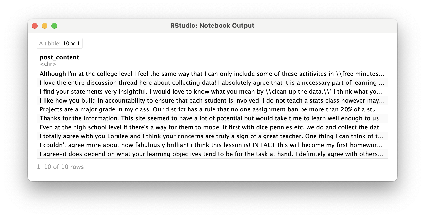
Use the filter() and grepl() functions introduced in Module 1. Section 3b to filter for rows in our ts_forum_data data frame that contain a term or terms of your choosing. Select a random sample of 10 posts using the sample_n() function for your term(s) and answer the questions below.

# A tibble: 10 × 1
   post_content                                                                 
   <chr>                                                                        
 1 "In my experience  students rarely find Statistics boring if the data we are…
 2 "I too enjoyed the School Census.  I think that this will be really helpful …
 3 "My goal for this course is to explore ideas on how to engage students explo…
 4 "Dear Awesome Teacher of Statistics  APOLOGIES FOR MULTIPLE POSTING DUE TO S…
 5 "It is amazing how quick we can recall things we learned years ago!  I somet…
 6 "aggree that integration of statistics into everyday experiences is essentia…
 7 "<p style=\\text-indent: -14px;\\\">  Airport Data     <ol><li>What learning…
 8 "It was an unique opportunity for me and I have learn a lot specifically fro…
 9 "Dear all   I am very happy to learn that so many online tools are available…
10 "At first I was not very interested in the Jane age investigation.  It lacke…

Your output should look something like this:

❓Questions

1. What, if anything, do these posts have in common?

   • YOUR RESPONSE HERE

2. What topics or themes might be apparent, or do you anticipate emerging, from our topic modeling?

   • YOUR RESPONSE HERE

Creating a Document Term Matrix

As highlighted in Chapter 5 of Text Mining with R, the {topicmodels} package and the Latent Dirichlet allocation (LDA) algorithm and LDA() function it uses expects document-term matrix as the data input.

Before we create a our document-term matrix, however, we have an important decision to make:

What do we consider to be a “document” in a MOOC-Ed discussion forum?

For example, we could consider each individual discussion post, or post_id in our data frame, as a document. It might also make sense to combine texts from all posts within each discussion, or disccussion_id, and consider that as our “document” since these posts are often interconnected an build off one another. For now, however, let treat each individual post as a unique document.

To create our document term matrix, we’ll need to first count() how many times each word occurs in each document, or post_id in our case, like so:

forums_tidy |>
  count(post_id, word) |>
  arrange(desc(n))

# A tibble: 142,641 × 3
   post_id word       n
   <chr>   <chr>  <int>
 1 20198   0        226
 2 50804   td       196
 3 20198   style    184
 4 34853   td       150
 5 20198   border   145
 6 20198   span     128
 7 20198   0px      126
 8 20198   color    125
 9 20198   rgb      124
10 20198   153      118
# ℹ 142,631 more rows

Once we have created a count of each word contained in a document, we next create a “tidy” matrix that contains one row per post as our original data frame did, but now contains a column for each word in the entire corpus and a value of n for how many times that word occurs in each post.

Let’s create this document term matrix from our post counts, we’ll use the cast_dtm() function and assign it to the variable forums_dtm:

forums_dtm <- forums_tidy |>
  count(post_id, word) |>
  cast_dtm(post_id, word, n)

👉 Your Turn ⤵

Use the code chunk below to print the forums_dtm object in the console and answer the following question:

print(forums_dtm)

<<DocumentTermMatrix (documents: 5766, terms: 13620)>>
Non-/sparse entries: 142641/78390279
Sparsity           : 100%
Maximal term length: NA
Weighting          : term frequency (tf)

1. What “class” of object is forums_dtm?
2. How many unique documents and terms are included our matrix?
3. Why might there be fewer documents/posts than were in our original data frame?
4. What exactly is meant by “sparsity”?

[1] "DocumentTermMatrix"    "simple_triplet_matrix"

<<DocumentTermMatrix (documents: 5766, terms: 13620)>>
Non-/sparse entries: 142641/78390279
Sparsity           : 100%
Maximal term length: NA
Weighting          : term frequency (tf)

2c. To Stem or not to Stem?

Next we’ll need to prepare our original data set for structural topic modeling using the textProcessor() function. The {stm} package has a number of features that extend the functionality of the topicmodels package, including an argument for “stemming” words, which Schofield and Mimno (2016) describe as follows:

Stemming is a popular way to reduce the size of a vocabulary in natural language tasks by conflating words with related meanings. Specifically, stemming aims to convert words with the same “stem” or root (e.g “creative” and “creator”) to a single word type (“create”). Though originally developed in the context of information retrieval (IR) systems, stemmers are now commonly used as a preprocessing step in unsupervised machine learning tasks.

The rationale behind stemming is that it can dramatically reduce the number of words or terms to be modeled, which in theory should help simplify and improve the performance of your model. We’ll explore this assumption a little later in this section.

Processing and Stemming for STM

Like unnest_tokens(), the textProcessor() function includes several useful arguments for processing text like converting text to lowercase and removing punctuation and numbers. I’ve included several of these in the script below along with their defaults used if you do not explicitly specify in your function. Most of these are pretty intuitive and you can learn more by viewing the ?textProcessor documentation.

Let’s go ahead and process our discussion forum post_content in preparation for our structural topic modeling that we’ll introduce later:

temp <- textProcessor(ts_forum_data$post_content, 
                    metadata = ts_forum_data,  
                    lowercase=TRUE, 
                    removestopwords=TRUE, 
                    removenumbers=TRUE,  
                    removepunctuation=TRUE, 
                    wordLengths=c(3,Inf),
                    stem=TRUE,
                    onlycharacter= FALSE, 
                    striphtml=TRUE, 
                    customstopwords=NULL)

Building corpus... 
Converting to Lower Case... 
Removing punctuation... 
Removing stopwords... 
Removing numbers... 
Stemming... 
Creating Output... 

Note that the first argument the textProcessor function expects is the column in our data frame that contains the text to be processed, in our case it’s the column post_content, which is extracted from ts_forum_data the using the $ operator.

The second argument metadata = expects the data frame that contains the text of interest and uses the column names to label the metadata such as course ids and forum names. This meatdata can be used to to improve the assignment of words to topics in a corpus and examine the relationship between topics and various covariates of interest.

Unlike the unnest_tokens() function, the output is not a nice tidy data frame. Topic modeling using the {stm} package requires a very unique set of inputs that are specific to the package. The following code will pull elements from the temp list that was created, which will be required for the stm() function we’ll use in Section 4:

meta <- temp$meta
vocab <- temp$vocab
docs <- temp$documents

Stemming Tidy Text

Notice that the textProcessor stem argument we used above is set to TRUE by default. We haven’t introduced word stemming at this point because there is some debate about the actual value of this process. Words like “students” and “student” might make sense to collapse into their base word and actually make analyses and visualizations more concise and easier to interpret. Hvitfeldt and Silge (2021) note, however, that words like the following have dramatic differences in meaning, semantics, and use and could result in poor models or misinterpreted results:

• meaning and mean
• likely, like, liking
• university and universe

The first word pair is particularly relevant to discussion posts from our Teaching Statistics course data. In addition, collapsing words like “teachers” and “teaching” could dramatically alter the results from a topic model.

Schofield and Mimno (2016) specifically noted that:

Despite their frequent use in topic modeling, we find that stemmers produce no meaningful improvement in likelihood and coherence and in fact can degrade topic stability.

For now, we will leave as is the forums_dtm we created earlier with words unstemmed, but what if we wanted to stem words in a “tidy” way?

Since the unnest_tokens() function does not (intentionally I believe) include a stemming function, one approach would be to use the wordStem() function from the snowballC package to either replace our words column with a word stems or create a new variable called stem with our stemmed words using the mutate() function.

Let’s do the latter and take a look at the original words and the stem that was produced:

stemmed_forums <- ts_forum_data |>
  unnest_tokens(output = word, input = post_content) |>
  anti_join(stop_words, by = "word") |>
  mutate(stem = wordStem(word))

stemmed_forums

# A tibble: 192,159 × 15
   course_id course_name       forum_id forum_name discussion_id discussion_name
   <chr>     <chr>             <chr>    <chr>      <chr>         <chr>          
 1 9         Teaching Statist… 126      Investiga… 6822          Not much compa…
 2 9         Teaching Statist… 126      Investiga… 6822          Not much compa…
 3 9         Teaching Statist… 126      Investiga… 6822          Not much compa…
 4 9         Teaching Statist… 126      Investiga… 6822          Not much compa…
 5 9         Teaching Statist… 126      Investiga… 6822          Not much compa…
 6 9         Teaching Statist… 126      Investiga… 6822          Not much compa…
 7 9         Teaching Statist… 126      Investiga… 6822          Not much compa…
 8 9         Teaching Statist… 126      Investiga… 6822          Not much compa…
 9 9         Teaching Statist… 126      Investiga… 6822          Not much compa…
10 9         Teaching Statist… 126      Investiga… 6822          Not much compa…
# ℹ 192,149 more rows
# ℹ 9 more variables: discussion_creator <dbl>, discussion_poster <dbl>,
#   discussion_reference <chr>, parent_id <dbl>, post_date <chr>,
#   post_id <chr>, post_title <chr>, word <chr>, stem <chr>

You can see that words like “activity” and “activities” that occur frequently in our discussions have been reduced to the word stem “activ”. If you are interested in learning other approaches for word stemming in R, as well as reading a more in depth description of the stemming process, I highly recommend the Chapter 4 Stemming from Hvitfeldt and Silge (2021) book, Supervised Machine Learning for Text Analysis in R.

👉 Your Turn ⤵

Complete the following code using what we learned in the section on Creating a Document Term Matrix and answer the questions below:

Hint: Make sure your code includes stem counts rather than word counts.

stemmed_dtm <- ts_forum_data |>
  unnest_tokens(output = word, input = post_content) |>
  anti_join(stop_words, by = "word") |>
  mutate(stem = wordStem(word)) |>
  ______() |>
  ______() |>
  
stemmed_dtm

<<DocumentTermMatrix (documents: 5766, terms: 10001)>>
Non-/sparse entries: 136185/57529581
Sparsity           : 100%
Maximal term length: NA
Weighting          : term frequency (tf)

<<DocumentTermMatrix (documents: 5766, terms: 13620)>>
Non-/sparse entries: 142641/78390279
Sparsity           : 100%
Maximal term length: NA
Weighting          : term frequency (tf)

# A tibble: 10,001 × 2
   stem         n
   <chr>    <int>
 1 student   7354
 2 data      4365
 3 statist   4161
 4 question  2470
 5 teach     1858
 6 class     1738
 7 school    1606
 8 time      1457
 9 learn     1372
10 font      1311
# ℹ 9,991 more rows

❓Questions

1. How many fewer terms are in our stemmed document term matrix?
   • YOUR RESPONSE HERE
2. Which words were clearly stemmed? Provide 3 examples:
   • EXAMPLE 1
   • EXAMPLE 2
   • EXAMPLE 3
3. Did stemming words significantly reduce the sparsity of the network?
   • YOUR RESPONSE HERE

3. MODEL

This module provides our first opportunity (VADER aside) for modeling text as data. In very simple terms, modeling involves developing a mathematical summary of a dataset. These summaries can help us further explore trends and patterns in our data.

In their book, Learning Analytics Goes to School, Krumm and Means Krumm, Means, and Bienkowski (2018) describe two general types of modeling approaches used in the Data-Intensive Research workflow: unsupervised and supervised learning. In distinguishing between the two, they note:

Unsupervised learning algorithms can be used to understand the structure of one’s dataset. Supervised models, on the other hand, help to quantify relationships between features and a known outcome. Known outcomes are also commonly referred to as labels or dependent variables.

In Section 3 we focus on Topic Modeling, an unsupervised learning approach to automatically identify topics in a collection of documents. In fact, we’ll explore two different approaches to topic modeling, as well as strategies for identifying the “right” number of topics:

1. Fitting a Topic Modeling with LDA. In this section we learn to use the {topicmodels} package and associated LDA() function for unsupervised classification of our forum discussions to find natural groupings of words, or topics.
2. Fitting a Structural Topic Model. We then explore the use of the {stm} package and stm() function to fit our model and uses metadata about documents to improve the assignment of words to “topics” in a corpus.
3. Choosing K. Finally, we wrap up Section 3 by learning about diagnostic properties like exclusivity, semantic coherence, and heldout likelihood for helping to select an appropriate number of topics.

3a. Fitting a Topic Modeling with LDA

Before running our first topic model using the LDA() function, let’s quick recap from our readings some basic principles behind Latent Dirichlet Allocation and why LDA is of preferred over other automatic classification or clustering approaches.

Unlike simple forms of cluster analysis such as k-means clustering, LDA is a “mixture” model, which in our context means that:

1. Every document contains a mixture of topics. Unlike algorithms like k-means, LDA treats each document as a mixture of topics, which allows documents to “overlap” each other in terms of content, rather than being separated into discrete groups. So in practice, this means that a discussion forum post could have an estimated topic proportion of 70% for Topic 1 (e.g. be mostly about a Topic 1), but also be partly about Topic 2.
2. Every topic contains a mixture of words. For example, if we specified in our LDA model just 2 topics for our discussion posts, we might find that one topic seems to be about pedagogy while another is about learning. The most common words in the pedagogy topic might be “teacher”, “strategies”, and “instruction”, while the learning topic may be made up of words like “understanding” and “students”. However, words can be shared between topics and words like “statistics” or “assessment” might appear in both equally.

Similar to k-means other other simple clustering approaches, however, LDA does require us to specify beforehand a value for k, i.e., the number of topics in our corpus. Selecting k is no trivial matter and can greatly impact your results.

Since we don’t have a have strong rationale about the number of topics that might exist in discussion forums, let’s use the n_distinct() function from the dplyr package to find the number of unique forum names in our course data and use that as a starting point:

n_distinct(ts_forum_data$forum_name)

[1] 21

Since it looks like there are about 20 distinct discussion forums, we’ll use that as our value for the k = argument of the LDA(). Be patient while this runs, since the default setting of is to perform a large number of iterations and can take several minutes to “fit” a model to the data.

n_distinct(ts_forum_data$forum_name)

[1] 21

forums_lda <- LDA(forums_dtm, 
                  k = 20,
                  method = "VEM",
                  control = list(seed = 588),
                  )

forums_lda

A LDA_VEM topic model with 20 topics.

Note that we used the control = argument to pass a random number (588) to seed the assignment of topics to each word in our corpus. Since LDA is a stochastic algorithm that could have different results depending on where the algorithm starts, specified a seed for reproducibility and so we’re all seeing the same results every time we specify the same number of topics.

By default, the LDA() function uses the method = “VEM” (Variational Expectation Maximization) estimation method, which is generally faster and more scalable. However, there is “Gibbs” (Gibbs Sampling) method, which is more accurate but computationally intensive, as well as the “CTM” (Correlated Topic Model) method, a variation of LDA with correlated topics.

Finally, tying back to our work in Module 1, Chris Bail (2020) notes that topic assignments for each word are updated in an iterative fashion and that LDA employs the Term Frequency-Inverse Document Frequency (TF-IDF) metric to assign probabilities.

Viewing Topic Terms

Before moving on, let’s view the top 5 words in each topic using the dead simple terms() function. We’ll also send this to the as_tibble() function to make the output a little easier to read:

terms(forums_lda, 5) |>
  as_tibble()

# A tibble: 5 × 20
  `Topic 1` `Topic 2`  `Topic 3` `Topic 4`  `Topic 5` `Topic 6`  `Topic 7` 
  <chr>     <chr>      <chr>     <chr>      <chr>     <chr>      <chr>     
1 dice      resources  students  statistics survey    stats      div       
2 fair      statistics kids      students   time      class      science   
3 trials    unit       nice      math       minutes   students   statistics
4 die       teaching   idea      teaching   idea      ap         sharing   
5 rolls     mooc       standard  teach      class     statistics students  
# ℹ 13 more variables: `Topic 8` <chr>, `Topic 9` <chr>, `Topic 10` <chr>,
#   `Topic 11` <chr>, `Topic 12` <chr>, `Topic 13` <chr>, `Topic 14` <chr>,
#   `Topic 15` <chr>, `Topic 16` <chr>, `Topic 17` <chr>, `Topic 18` <chr>,
#   `Topic 19` <chr>, `Topic 20` <chr>

👉 Your Turn ⤵

Use the code chunk below to increase the number of terms associated with each “Topic” and answer the prompt that follows:

terms(forums_lda, 10) |>
  as_tibble()

# A tibble: 10 × 20
   `Topic 1`  `Topic 2`  `Topic 3`  `Topic 4`   `Topic 5` `Topic 6`  `Topic 7`  
   <chr>      <chr>      <chr>      <chr>       <chr>     <chr>      <chr>      
 1 dice       resources  students   statistics  survey    stats      div        
 2 fair       statistics kids       students    time      class      science    
 3 trials     unit       nice       math        minutes   students   statistics 
 4 die        teaching   idea       teaching    idea      ap         sharing    
 5 rolls      mooc       standard   teach       class     statistics students   
 6 rolling    ideas      understand school      semester  school     love       
 7 unfair     learning   language   level       student   math       http       
 8 6          teachers   agree      teachers    worry     teach      mathematics
 9 conclusion activities deviation  mathematics sites     college    class      
10 roll       learn      english    agree       sleep     project    teachers   
# ℹ 13 more variables: `Topic 8` <chr>, `Topic 9` <chr>, `Topic 10` <chr>,
#   `Topic 11` <chr>, `Topic 12` <chr>, `Topic 13` <chr>, `Topic 14` <chr>,
#   `Topic 15` <chr>, `Topic 16` <chr>, `Topic 17` <chr>, `Topic 18` <chr>,
#   `Topic 19` <chr>, `Topic 20` <chr>

As you can see form the output, each “Topic” is essentially a “bag-of-words” that typically occur together across documents. Pick two topics from the table above and use a short phrase or sentence that you think describes the topic.

• TOPIC X: YOUR DESCRIPTION HERE

• TOPIC X: YOUR DESCRIPTION HERE

3b. Fitting a Structural Topic Model

Bail notes that LDA, while perhaps the most common approach to topic modeling, is just one of many different types, including Dynamic Topic Models, Correlated Topic Models, Hierarchical Topic Models, and more recently, Structural Topic Modeling (STM). He argues that one reason STM has risen in popularity and use is that it employs meta data about documents to improve the assignment of words to topics in a corpus and can be used to examine relationships between covariates and documents.

Also, since Julia Silge has indicated that STM is, “my current favorite implementation of topic modeling in R” and has built supports in the tidytext package for building structural topic models, this package is definitely worth discussing in this case study. I also highly recommend her own case study of the stm package: The game is afoot! Topic modeling of Sherlock Holmes stories as well as her follow up post, Training, evaluating, and interpreting topic models.

Note

LLM-Based Approaches to Topic Modeling

Large Language Models (LLMs), such as GPT-4, BERT, and T5, which leverage deep learning and contextual embeddings, have also emerged as promising approaches for modeling topics within a corpus. Unlike traditional Latent Dirichlet Allocation (LDA), LLM-based topic modeling approaches and libraries such as {BERTopic} use pre-trained transformers, embeddings, and clustering techniques to extract meaningful topics.

The stm Package

As we’ve seen above, STM uses an unusual temp textProcessor output that is unique to the stm package. And as you’ve probably already guessed, the stm() function for fitting a structural topic model does not take a fairly standard document term matrix like the LDA() function.

Before we fit our model, we’ll have to extract the elements from the temp object created after we processed our text. Specifically, the stm() function expects the following arguments:

• documents = the document term matrix to be modeled in the native stm format
• data = an optional data frame containing meta data for the prevalence and/or content covariates to include in the model
• vocab = a character vector specifying the words in the corpus in the order of the vocab indices in documents.

Let’s go ahead and extract these elements:

docs <- temp$documents 
meta <- temp$meta 
vocab <- temp$vocab 

And now use these elements to fit the model using the same number of topics for K that we specified for our LDA topic model. Let’s also take advantage of the fact that we can include the course_id and forum_id covariates in the prevealence = argument to help improve, in theory, our model fit:

forums_stm <- stm(documents=docs, 
         data=meta,
         vocab=vocab, 
         prevalence =~ course_id + forum_id,
         K=20,
         max.em.its=25,
         verbose = FALSE)

forums_stm

A topic model with 20 topics, 5781 documents and a 7820 word dictionary.

As noted earlier, the stm package has a number of handy features. One of these is the plot.STM() function for viewing the most probable words assigned to each topic.

By default, it only shows the first 3 terms so let’s change that to 5 to help with interpretation:

plot.STM(forums_stm, n = 5)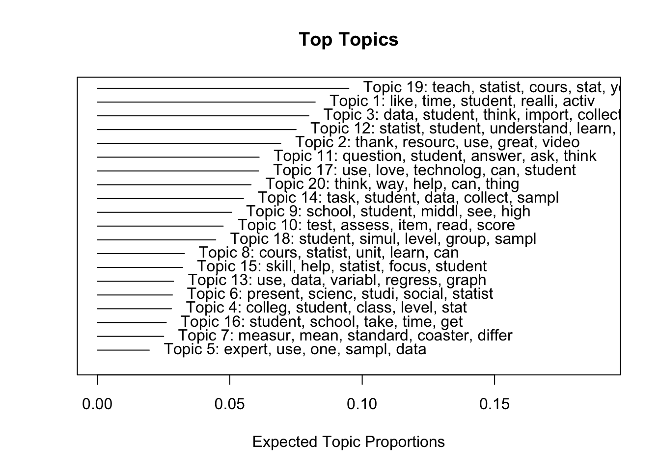

Note that you can also just use the base R plot() function as well:

plot(forums_stm, n = 5)

You should see an output that looks something like the image below:

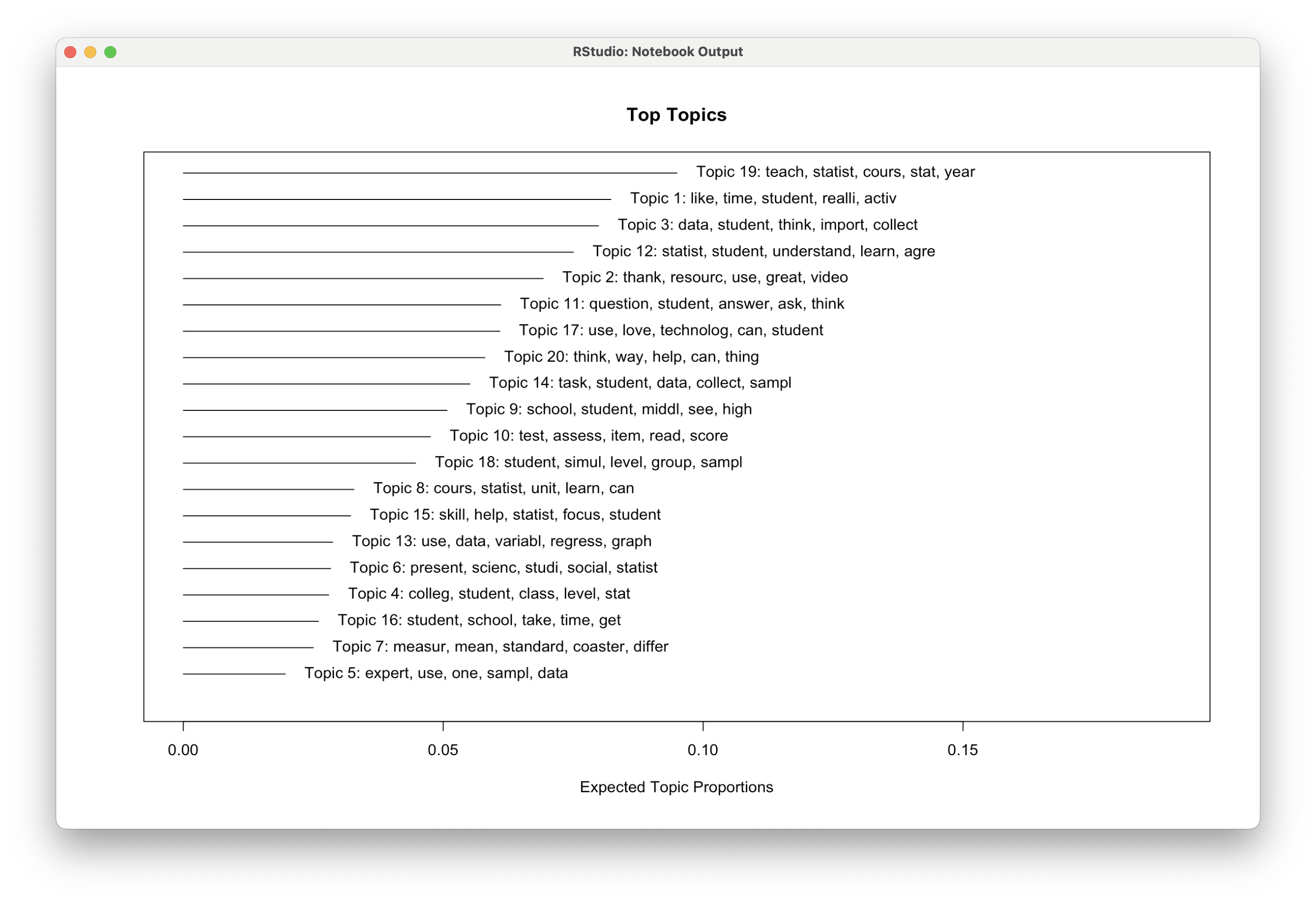
Let’s break down what we’re seeing:

• Title: “Top Topics”

  • This indicates that the visualization represents the most prominent topics identified by the STM model.

• Topic Labels and Keywords

  • Each topic is listed as Topic X (e.g., Topic 19, Topic 1, etc.), followed by its most representative words.

  • The words are stemmed (e.g., statist → statistics, cours → course), indicating preprocessing steps such as stemming or lemmatization.

  • The keywords reflect the semantic content, or “signature,” of each topic and provide a snapshot of what each topic represents.

• Horizontal Bars

  • Each horizontal bar represents the expected topic proportion, i.e., how prevalent each topic is in the corpus, i.e., our entire body of posts.

  • The longer the bar, the more dominant the topic is across documents.

• X-Axis: “Expected Topic Proportions”

  • This represents the proportion of the dataset that each topic occupies.

  • Topics with higher proportions are more frequently discussed in the corpus.

👉 Your Turn ⤵

Fit a model for both LDA and STM using different values for K and answer the questions below:

# YOUR CODE HERE

1. What topics appear to be similar to those using 20 topics for K?
   • YOUR RESPONSE HERE
2. Knowing that you don’t have as much context as I do, how might you interpret one of these latent topics or themes using the key terms assigned?
   • YOUR RESPONSE HERE
3. What topic emerged that seem dramatically different and how might you interpret this topic?
   • YOUR RESPONSE HERE

3c. Finding K

As alluded to earlier, selecting the number of topics for your model is a non-trivial decision and can dramatically impact your results. Bail (2018) notes that

The results of topic models should not be over-interpreted unless the researcher has strong theoretical apriori about the number of topics in a given corpus, or if the researcher has carefully validated the results of a topic model using both the quantitative and qualitative techniques described above.

There are several approaches to estimating a value for K and we’ll take a quick look at one from the {ldatuning} package and one from our stm package.

The FindTopicsNumber() Function

The {ldatuning} package has functions for both calculating and plotting different metrics that can be used to estimate the most preferable number of topics for LDA model. It also conveniently takes the standard document term matrix object that we created from out tidy text and has the added benefit of running fairly quickly, especially compared to the function for finding K from the {stm} package.

Let’s use the defaults specified in the ?FindTopicNumber documentation and modify slightly get metrics for a sequence of topics from 10-75 counting by 5 and plot the output we saved using the FindTopicsNumber_plot() function:

k_metrics <- FindTopicsNumber(
  forums_dtm,
  topics = seq(10, 75, by = 5),
  metrics = "Griffiths2004",
  method = "Gibbs",
  control = list(),
  mc.cores = NA,
  return_models = FALSE,
  verbose = FALSE,
  libpath = NULL
)

FindTopicsNumber_plot(k_metrics)

Note that the FindTopicNumbers() function contains three additional metrics for calculating metrics that can be used to estimate the most preferable number of topics for LDA model. We used the Griffiths2004 metrics included in the default example and I’ve also found this to produce the most interpretable results as show in the figure below:

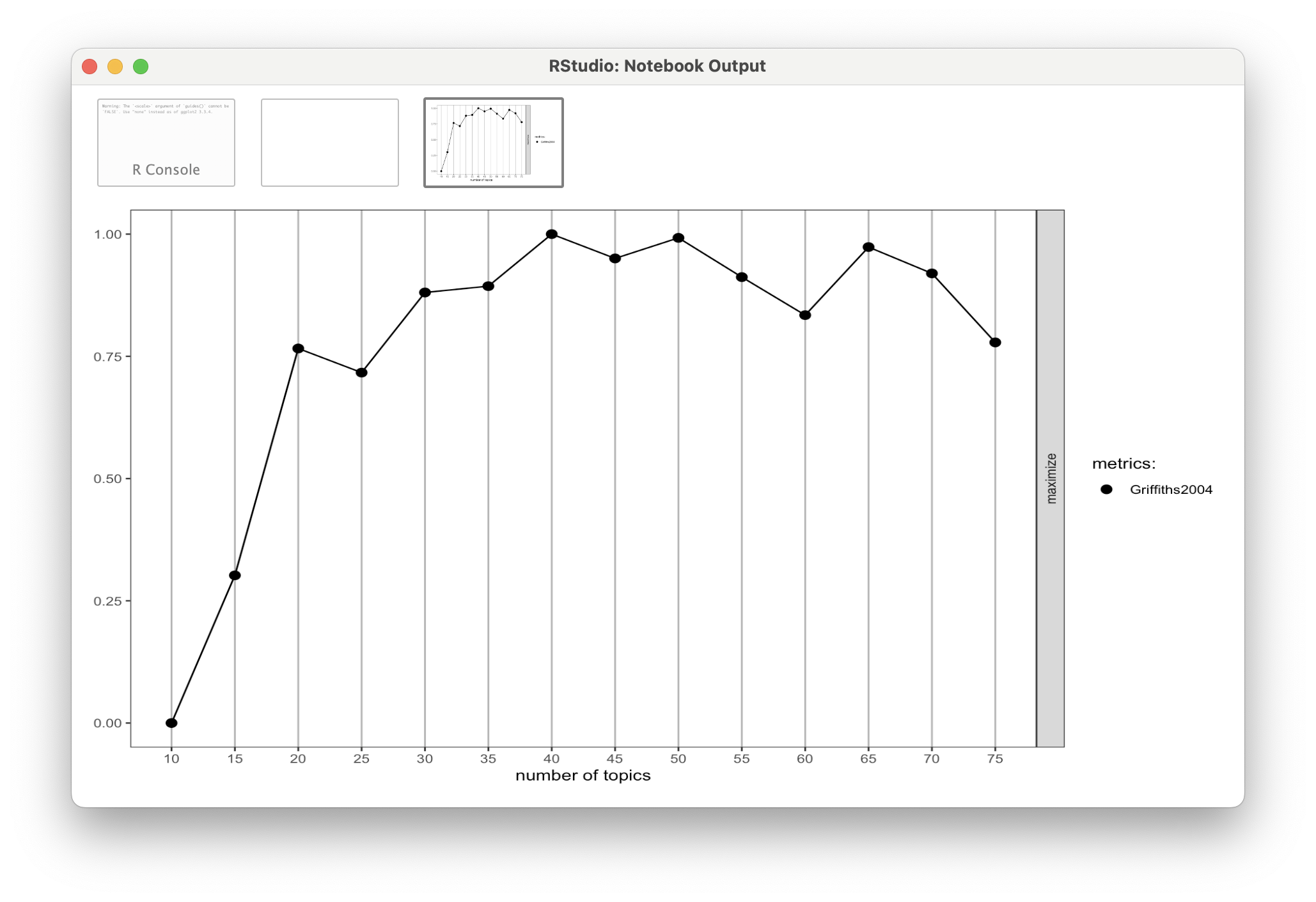
As a general rule of thumb and overly simplistic heuristic, we’re looking for an inflection point in our plot which indicates an optimal number of topics to select for a value of K.

The findingK() Function

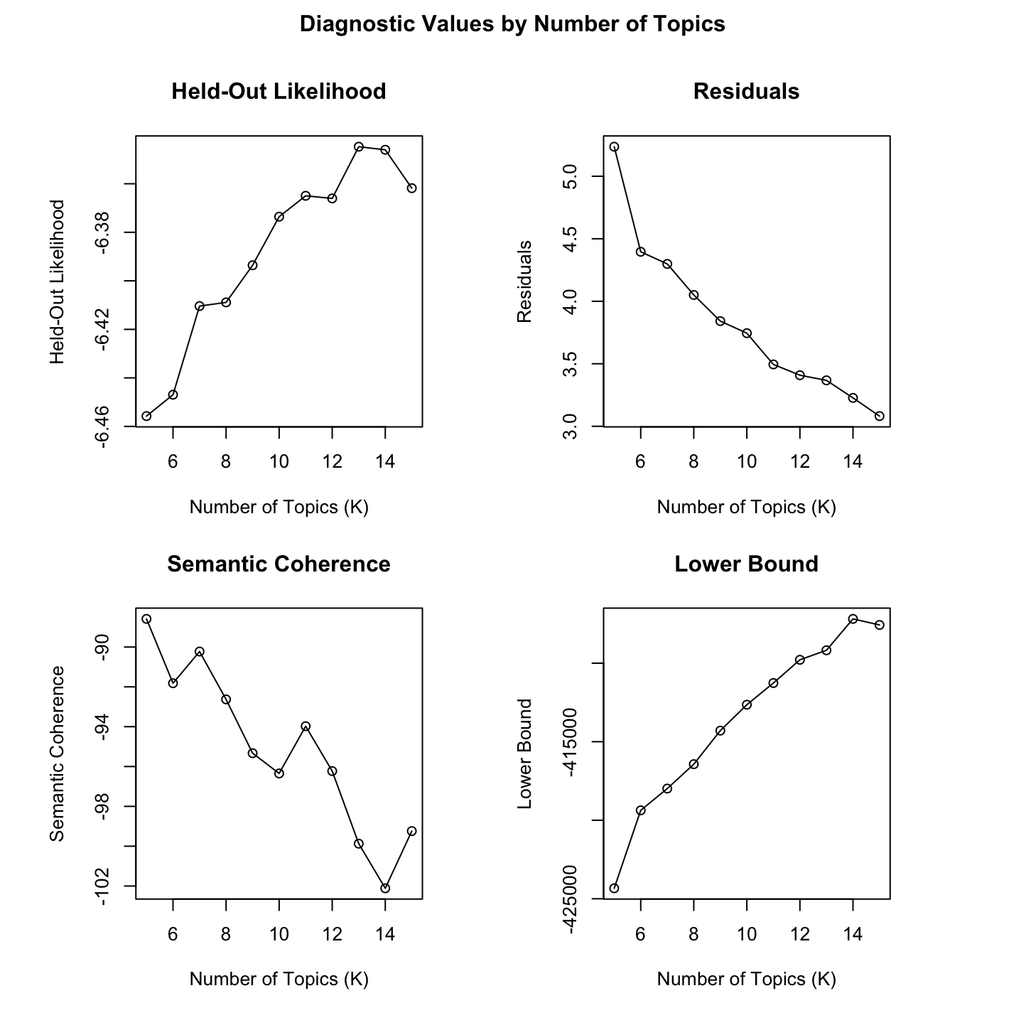
Finally, Bail (2018) notes that thestm package has a useful function called searchK which allows us to specify a range of values for k and outputs multiple goodness-of-fit measures that are “very useful in identifying a range of values for k that provide the best fit for the data.”

The syntax of this function is very similar to the stm() function we used above, except that we specify a range for k as one of the arguments. In the code below, we search all values of k between 10 and 30.

findingk <- searchK(docs, 
                    vocab, 
                    K = c(5:15),
                    data = meta, 
                    verbose=FALSE)

plot(findingk)

Warning

Computationally Intensive!

Note that running the searchK() function on this corpus took all night on a pretty powerful MacBook Pro and crashed once as well, so I do not expect you to run this for the case study.

After a couple iterations searchK() landed on between 5 and 15 with an optimal number of topics somewhere around 14:

Given the somewhat conflicting results – also somewhat selfishly and for the same of simplicity for this case study – I’m just going to stick with the rather arbitrary selection of 20 topics for the remainder of this case study.

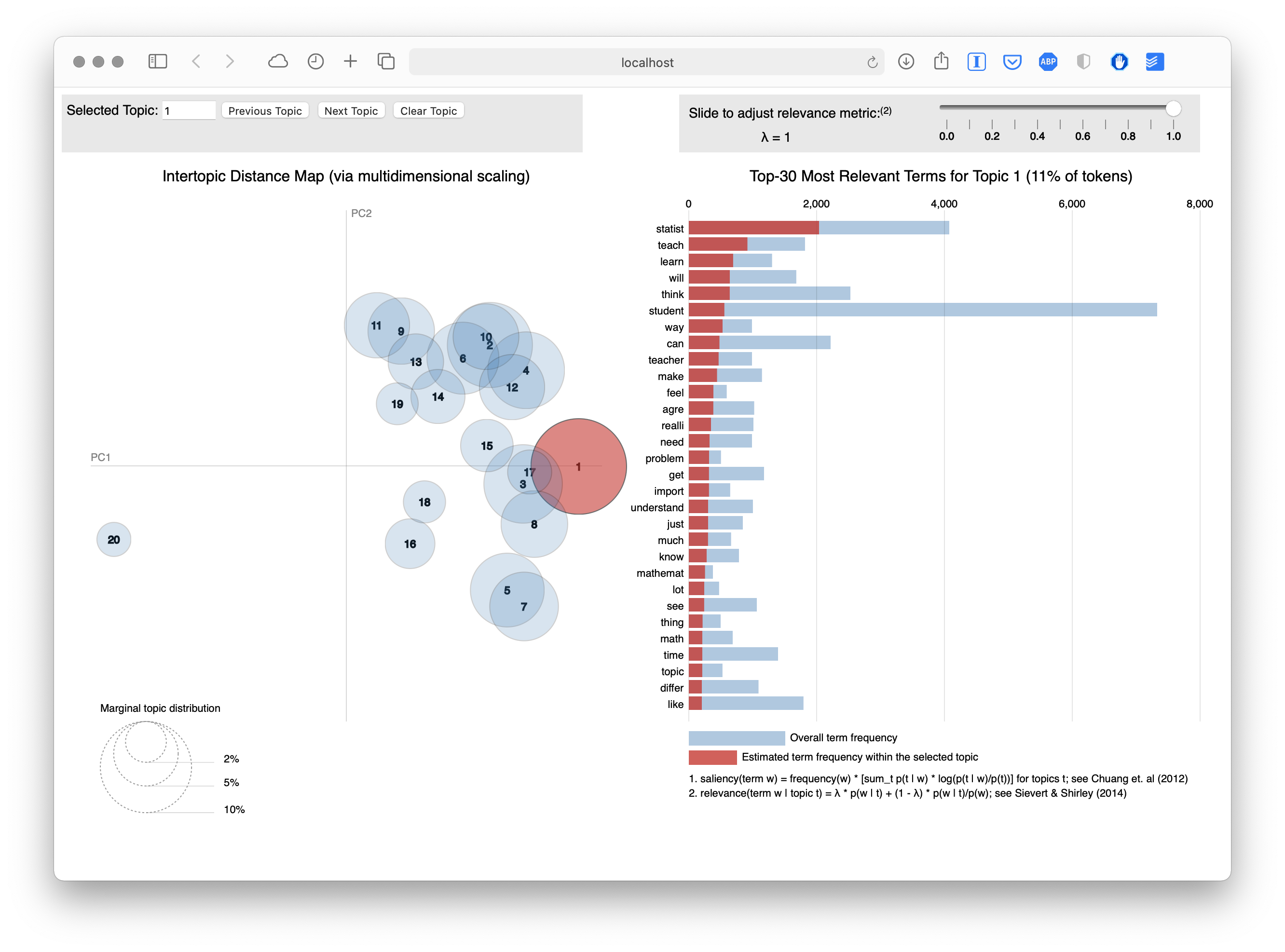
The LDAvis Explorer

One final tool that I want to introduce from the stm package is the toLDAvis() function which provides a great visualizations for exploring topic and word distributions using LDAvis topic browser:

toLDAvis(mod = forums_stm, docs = docs)

Loading required namespace: servr

As you can see from the browser screen shot below, our current STM with 20 topics is resulting in a lot of overlap among topics and suggest that 20 may not be an optimal number of topics, as other approaches for finding k also suggests:

4. EXPLORE

Silge and Robinson (2018) note that fitting at topic model is the “easy part.” The hard part is making sense of the model results and that the rest of the analysis involves exploring and interpreting the model using a variety of approaches which we’ll case study in in this section.

Bail (2018) cautions, however, that:

…post-hoc interpretation of topic models is rather dangerous… and can quickly come to resemble the process of “reading tea leaves,” or finding meaning in patterns that are in fact quite arbitrary or even random.

4a. Exploring Beta Values

Hidden within this forums_lda topic model object we created are per-topic-per-word probabilities, called β (“beta”). It is the probability of a term (word) belonging to a topic. 

Let’s take a look again at the 5 most likely terms assigned to each topic, i.e. those with the largest β values using the terms() function from the topicmodels package:

terms(forums_lda, 5) |>
  as_tibble()

# A tibble: 5 × 20
  `Topic 1` `Topic 2`  `Topic 3` `Topic 4`  `Topic 5` `Topic 6`  `Topic 7` 
  <chr>     <chr>      <chr>     <chr>      <chr>     <chr>      <chr>     
1 dice      resources  students  statistics survey    stats      div       
2 fair      statistics kids      students   time      class      science   
3 trials    unit       nice      math       minutes   students   statistics
4 die       teaching   idea      teaching   idea      ap         sharing   
5 rolls     mooc       standard  teach      class     statistics students  
# ℹ 13 more variables: `Topic 8` <chr>, `Topic 9` <chr>, `Topic 10` <chr>,
#   `Topic 11` <chr>, `Topic 12` <chr>, `Topic 13` <chr>, `Topic 14` <chr>,
#   `Topic 15` <chr>, `Topic 16` <chr>, `Topic 17` <chr>, `Topic 18` <chr>,
#   `Topic 19` <chr>, `Topic 20` <chr>

Even though we’ve somewhat arbitrarily selected the number of topics for our corpus, some these topics or themes are fairly intuitive to interpret. For example:

• Topic 11 (technology, students, software, program, excel) seems to be about students use of technology including software programs like excel;

• Topic 9 (questions, kids, love, gapminder, sharing) seems to be about the gapminder activity from the MOOC-Ed and kids enjoyment of it; and

• Topic 18 (data, students, collect, real, sets) seems to be about student collection and use of real world data sets.

Not surprisingly, the tidytext package has a handy function conveniently name tidy() to convert our LDA model to a tidy data frame containing these beta values for each term:

tidy_lda <- tidy(forums_lda)

tidy_lda

# A tibble: 272,400 × 3
   topic term       beta
   <int> <chr>     <dbl>
 1     1 2015  4.61e-267
 2     2 2015  1.05e-  3
 3     3 2015  4.93e- 42
 4     4 2015  1.20e- 63
 5     5 2015  2.55e- 30
 6     6 2015  7.84e- 35
 7     7 2015  8.17e- 33
 8     8 2015  6.25e- 33
 9     9 2015  1.10e-  4
10    10 2015  6.75e-  5
# ℹ 272,390 more rows

Obviously, it’s not very easy to interpret what the topics are about from a data frame like this so let’s borrow code again from Chapter 8.4.3 Interpreting the topic model in Text Mining with R to examine the top 5 terms for each topic and then look at this information visually:

top_terms <- tidy_lda |>
  group_by(topic) |>
  slice_max(beta, n = 5, with_ties = FALSE) |>
  ungroup() |>
  arrange(topic, -beta)

top_terms |>
  mutate(term = reorder_within(term, beta, topic)) |>
  group_by(topic, term) |>    
  arrange(desc(beta)) |>  
  ungroup() |>
  ggplot(aes(beta, term, fill = as.factor(topic))) +
  geom_col(show.legend = FALSE) +
  scale_y_reordered() +
  labs(title = "Top 5 terms in each LDA topic",
       x = expression(beta), y = NULL) +
  facet_wrap(~ topic, ncol = 4, scales = "free")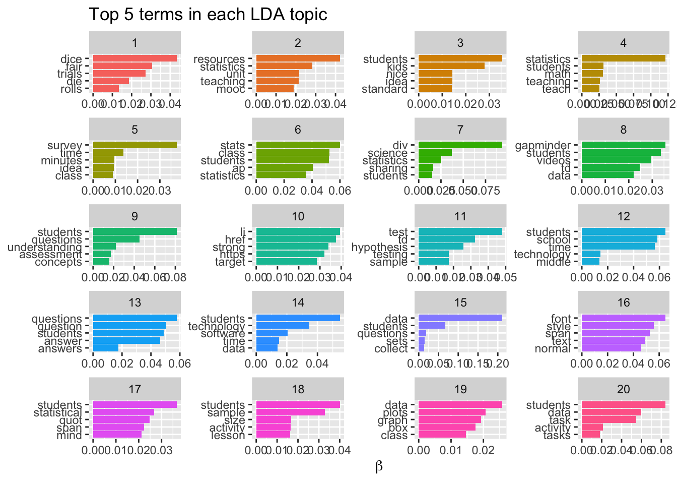

4b. Exploring Gamma Values

Now that we have a sense of the most common words associated with each topic, let’s take a look at the topic prevalence in our MOOC-Ed discussion forum corpus, including the words that contribute to each topic we examined above.

Also, hidden within our forums_lda topic model object we created are per-document-per-topic probabilities, called γ (“gamma”). This provides the probabilities that each document is generated from each topic, that gamma matrix. We can combine our beta and gamma values to understand the topic prevalence in our corpus, and which words contribute to each topic.

To do this, we’re going to again borrow some code from the Silge (2018) post, Training, evaluating, and interpreting topic models.

First, let’s create two tidy data frames for our beta and gamma values

td_beta <- tidy(forums_lda)

td_gamma <- tidy(forums_lda, matrix = "gamma")

td_beta

# A tibble: 272,400 × 3
   topic term       beta
   <int> <chr>     <dbl>
 1     1 2015  4.61e-267
 2     2 2015  1.05e-  3
 3     3 2015  4.93e- 42
 4     4 2015  1.20e- 63
 5     5 2015  2.55e- 30
 6     6 2015  7.84e- 35
 7     7 2015  8.17e- 33
 8     8 2015  6.25e- 33
 9     9 2015  1.10e-  4
10    10 2015  6.75e-  5
# ℹ 272,390 more rows

td_gamma

# A tibble: 115,320 × 3
   document topic    gamma
   <chr>    <int>    <dbl>
 1 11295        1 0.00196 
 2 12711        1 0.000248
 3 12725        1 0.0262  
 4 12733        1 0.00229 
 5 12743        1 0.00777 
 6 12744        1 0.00391 
 7 12756        1 0.0262  
 8 12757        1 0.00289 
 9 12775        1 0.00289 
10 12816        1 0.00289 
# ℹ 115,310 more rows

Next, we’ll adopt Julia’s code wholesale to create a filtered data frame of our top_terms, join this to a new data frame for gamma-terms and create a nice clean table using the kabel() function knitr package:

top_terms <- td_beta |>
  arrange(beta) |>
  group_by(topic) |>
  top_n(7, beta) |>
  arrange(-beta) |>
  select(topic, term) |>
  summarise(terms = list(term)) |>
  mutate(terms = map(terms, paste, collapse = ", ")) |> 
  unnest()

Warning: `cols` is now required when using `unnest()`.
ℹ Please use `cols = c(terms)`.

gamma_terms <- td_gamma |>
  group_by(topic) |>
  summarise(gamma = mean(gamma)) |>
  arrange(desc(gamma)) |>
  left_join(top_terms, by = "topic") |>
  mutate(topic = paste0("Topic ", topic),
         topic = reorder(topic, gamma))

gamma_terms |>
  select(topic, gamma, terms) |>
  kable(digits = 3, 
        col.names = c("Topic", "Expected topic proportion", "Top 7 terms"))

Topic	Expected topic proportion	Top 7 terms
Topic 4	0.087	statistics, students, math, teaching, teach, school, level
Topic 2	0.080	resources, statistics, unit, teaching, mooc, ideas, learning
Topic 9	0.079	students, questions, understanding, assessment, concepts, test, statistical
Topic 6	0.078	stats, class, students, ap, statistics, school, math
Topic 15	0.078	data, students, questions, sets, collect, question, real
Topic 20	0.070	students, data, task, activity, tasks, question, cycle
Topic 14	0.064	students, technology, software, time, data, agree, real
Topic 13	0.059	questions, question, students, answer, answers, correct, results
Topic 8	0.053	gapminder, students, videos, td, data, video, site
Topic 12	0.049	students, school, time, technology, middle, video, student
Topic 3	0.045	students, kids, nice, idea, standard, understand, language
Topic 18	0.038	students, sample, size, activity, lesson, data, results
Topic 17	0.038	students, statistical, quot, span, mind, level, reasoning
Topic 7	0.033	div, science, statistics, sharing, students, love, http
Topic 11	0.033	test, td, hypothesis, testing, sample, difference, results
Topic 19	0.030	data, plots, graph, box, class, median, plot
Topic 10	0.030	li, href, strong, https, target, _blank, statistics
Topic 16	0.023	font, style, span, text, normal, 0px, color
Topic 5	0.020	survey, time, minutes, idea, class, semester, student
Topic 1	0.014	dice, fair, trials, die, rolls, rolling, unfair

And let’s also compare this to the most prevalent topics and terms from our forums_stm model that we created using the plot() function:

plot(forums_stm, n = 7)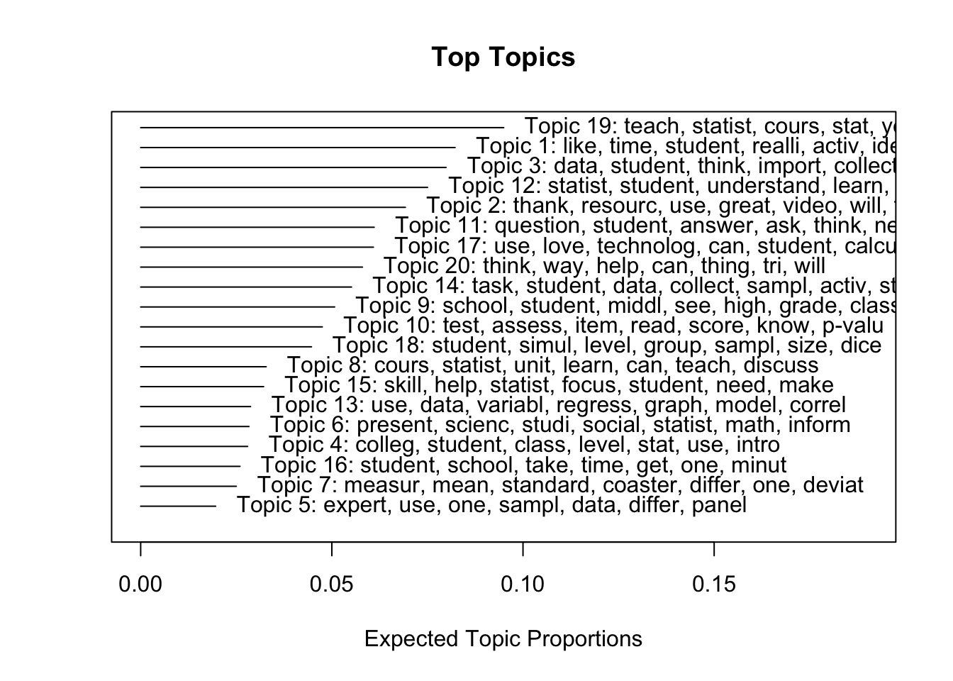

4c. Reading the Tea Leaves

Recognizing that topic modeling is best used as a “tool for reading” and provides only an incomplete answer to our overarching, “How do we quantify what a corpus is about?”, the results do suggest some potential topics that have emerged, as well as some areas worth following up on.

Specifically, looking at some of the common clusters of words for the more prevalent topics suggest that some key topics or “latent themes” (renamed in bold) might include:

• Teaching Statistics: Unsurprising, given the course title, the topics most prevalent in both the forums_stm and forums_lda models contains the terms “teach”, “students”, “statistics”. This could be an “overarching theme” but more likely may simply just be residue from the course title being sprinkled throughout the forums and deserves some follow up. Topics 8 from the LDA model may overlap with this topic as well.
• Course Utility: The second most prevalent Topics (13 and 2) in the lda and stm models respectively, seem to potentially be about the usefulness of course “resources” like lessons, tools, videos, and activities. I’m wagering this might be a forum dedicated to course feedback. Topic 15 from the STM model also suggest this may be a broader theme.
• Using Real-World Data: Topics 18 & 12 from the LDA model particularly intrigued me and I’m wagering this is pretty positive sentiment among participants about the value and benefit of having students collect and analyze real data sets (e.g. Census data in Topic 1) and work on projects relevant to their real life. Will definitely follow up on this one.
• Technology Use: Several topics (6 & 11 from LDA and 8 & 19 from STM) appear to be about student use of technology and software like calculators and Excel for teaching statistics and using simulations. Topic 16 from LDA also suggest the use of the Common Online Data Analysis Platform (CODAP).
• Student Struggle & Engagement: Topic 15 from LDA and Topic 16 from STM also intrigue me and appear to be two opposite sides of perhaps the same coin. The former includes “struggle” and “reading” which suggests perhaps a barrier to teaching statistics while Topic 16 contains top stems like “engage”, “activ”, and “think” and may suggest participants anticipate activities may engage students.

To serve as a check on my tea leaf reading, I’m going to follow Bail’s recommendation to examine some of these topics qualitatively. The stm package has another useful (though exceptionally fussy) function called findThoughts which extracts passages from documents within the corpus associate with topics that you specify.

The first line of code may not be necessary for your independent analysis, but because the textProcessor() function removed several documents during processing, the findthoughts() function can’t properly index the processed docs. This line of code found on stackoverflow removes documents from original ts_forum_data source that were removed during processing so there is a one-to-one correspondence with forums_stm and so you can use the function to find posts associated with a given topic.

Let’s slightly reduce our original data set to match our STM model, pass both to the findThoughts() function, and set our arguments to return n =10 posts from topics = 2 (i.e. Topic 2) that have at least 50% or thresh = 0.5 as a minimum threshold for the estimated topic proportion.

ts_forum_data_reduced <-ts_forum_data$post_content[-temp$docs.removed]

findThoughts(forums_stm,
             texts = ts_forum_data_reduced,
             topics = 2, 
             n = 10,
             thresh = 0.5)

 Topic 2: 
     Thank you for providing these links and resources. The resources you provided in this MOOC have been very beneficial. I look forward to utilizing them in future lessons.
    Ronald-  We are glad that you have identied resources that you want to return to. If you do bookmark the urls they are available on the web after the course is closed.
    Thank you for sharing this resource.  I look forward to exploring it further.
    My students use iNZight a lot  which is free  and is a less cumbersome  more student-friendly version of R:  https://www.stat.auckland.ac.nz/~wild/iNZight/index.php  The online version is also available:  http://docker.stat.auckland.ac.nz/
    will download a preview to explore it. Thank you for the recommendation.
    I would download all pdfs and bookmark sites you might want in the future.
    Thanks for the info.  I will definitely download many of the resources I liked for future use.  Having a bank of resources for statistics is crucial.
    I'll add my voice to the chorus of gratitude.  I've already used a couple of the activities presented here in my fall quarter course  and I will definitely bookmark as many of the resources as possible to try to use in the future.  Thank you!
    Thank you for sharing!  I look forward to using this in my class.
    Great resource  thanks for sharing!

Duplicate posts aside, this Course Utility topic returns posts there were expected based on my interpretation of the key terms for Topic 2. It looks like I may have read those tea leaves correctly!

Now let’s take a look at Topic 16 that we thought might be related to student engagement:

findThoughts(forums_stm,
             texts = ts_forum_data_reduced,
             topics = 16, 
             n = 10,
             thresh = 0.5)

 Topic 16: 
     Hi Folks   One of the discussions that needs to occur when studying the travel time of walking vs. driving by car vs riding on a school bus is the number of stops the bus must make in order to pick up students.  One of my previous careers was that of a school bus driver.  At each stop I was required to stop the bus  put on the flashing lights  put on the emergency brake  look through all of the mirrors to determine all of the cars had stopped  open the bus door  then pick up the microphone (which could be heard inside and outside of the bus) to tell the students it was now safe to cross the road and enter the bus.  After waiting for all students to get on the bus and take a seat and for the bus monitor to check under the bus and get on the bus again; I would then close the bus door and take off the emergency brake.  Next  I would check all of my mirrors to make sure it was safe pull completely back into the lane of travel and continue on my bus route. All of these actions increased the amount of time it took to get to school.  What is the purpose of this investigation?  I would want to know if the students with the longer travel time to and from school are impacted by the amount of time spent traveling each day.  What are the grades of the students with the longest travel time how do those grades compare to students with the least travel time? What behaviors are exhibited by students in school who spend the most time traveling to and from school? Are they more likely to exhibit behaviors that result in disciplinary referrals? Does travel time negatively impact the academic and behavioral performance of these students in school? On the flip slide  does longer travel time provide the opportunity for students to engage in preferred activities of talking to their friends on the bus or engaging in their electronic device to listen to music or play games and does this provide a beginning and end of the day relaxation experience for the students. Do these students have better grades and less disciplinary referrals?
    A couple of other thoughts I had on the travel times as I went through the videos:  1. I did ask students about travel time one year and observed an interesting tendency for the very short travel times e.g. 5 minutes  8 minutes  12 minutes  to be reported with higher accuracy than longer travel times e.g. 60 minutes  775 minutes  90 minutes.  2. I wonder about the day-to-day variability that is hidden when students report  as they do here  a \typical\" travel time. I used to walk to university and once I had established that the walk took about 35 minutes  I could speed up or slow down so that my walk time took about 35 minutes every single day  as I would leave home 36 minutes before my first class every day! The point being  that a walk time is likely to be less variable than a car or bus time  as well as being shorter on average.  "
    In the county system that I teach in  students live several miles away from our rural school.  They can ride a bus for 20 minutes or more before the 1st stop.  Some parents choose to bring their kids to school due to behaviors on buses or lengths of time their child would have to be on a bus.  None of our students walk to school.
    These machine-generated animations bug me.  Is there any evidence that they are at least a non-issue to students?  I'm so annoyed by the stilted speech and missing limbs that I'd be hard pressed to grapple with fresh content too.
    Nina   Each state has an average teacher salary  so we're comparing average teacher salaries from state to state. Therefore  each state's average becomes a single value that we're comparing. It doesn't matter that some states are bigger or smaller since it's the average that we're comparing.    If we wanted to get the national average  then yes  we would have to take into account the number of teachers for each state. In that case  we would look at the frequency distribution (each state average and # of teachers) to calculate the overall  or national average.
    The Statkey home website has a ton of csv files and other formats too.  I haven't tried it  but I bet at least one of the file types would work.<table border=\1\" cellspacing=\"0\" cellpadding=\"1\" width=\"420\"><tbody><tr><td> CSV</td><td>Excel</td><td>ASCII</td><td>  R  </td><td>Minitab</td><td>Fathom</td><td>  JMP</td></tr></tbody></table>   http://www.lock5stat.com/datapage.html        "
    Beverly   I used the animations with preservice teachers. Since my animation was short and it was their first time watching one we watched it once just for them to laugh at the speech and missing limbs. But after that we watched it again and they took it seriously and it wasn't a problem since they knew it was made from students' real work. Also  a few of the animations in the MOOC of real voices. Do you like those better? Those just take a little longer since you have to get kids to volunteer! :)
    Hi MIchelle  I too found the Gapminder and the someone named Jane quite compelling. What intrigued me was the variety of approaches each student implemented to answer the question.  Furthermore  I googled the top 20 fave people named Ralph  were Ralph Lauren and Ralph Fiennes.
    Have you looked at the BrainPop videos?  They are all animations and the students like them so much.  I think student thinking has evolved over the past 10 years.  Ten years ago my students found the Brain Pop videos as annoying as I do.  Now they always want more.  It must be that digital native orientation to life.
    I just saved the entire page to my documents folder so I could draw on repeatedly next year.

It looks like my tea reading was a partially correct for Topic 16, though the results seem to be about a specific “Pepsi challenge” activity conducted with students.

Finally, let’s look at posts from Topic 3 which we though might be an overarching theme about teaching statistics:

ts_forum_data_reduced <-ts_forum_data$post_content[-temp$docs.removed]

findThoughts(forums_stm,
             texts = ts_forum_data_reduced,
             topics = 3, 
             n = 10,
             thresh = 0.5)

 Topic 3: 
     I think a crucial thing for students to identify is where the data is coming from and how it was collected. Without knowing the origins of the data is important for students to remain skeptical about how realistic the results are that the data is implying. This mindset is important for students to employ especially when they apply it to their daily lives such as when looking at surveys and data results in newspapers. It's important to look at who collected the data and the reasons behind collecting. This may lead to realization that the people collecting the data may be pushing you towards a certain conclusion.
    This is an interesting conversation thread. I see the value in exposing students to relevant  serious datasets. Learning to pose questions  clean data  analyze real data  and interpret results in the context of a real problem is one of the most valuable experiences a statistician should undergo. However  many of the real  societally-relevant datasets contain so many variables and observations that a K-12 student would be easily overwhelmed.   Having students collect data on shoe size  or some other 'fun' constructed task would yield a dataset that is much easier to deal with in a classroom setting. Many students might become interested in statistics from such exercises.  How do you think you could make serious  real-world problems accessible to students at all levels?   One possibility would be to take a subset of real-world data  do a bit of data cleaning  and present the subset of data to students. I do believe that many students are motivated by important  relevant problems  but those problems should be presented at an appropriate level.
    Our textbook also instructs to analyze data with and without outliers.  I think students can then say \Here's what the data indicates\" and then be skeptical and say they are suspicious of certain data points and why and analyze the data without outliers.  That allows our students to think critically and be skeptical  while still being objective.  "
    I had the aha moment that context is crucial and how data was collected was crucial.
    I agree with you on the importance of cleaning up data.  Our curriculum in NYS has always been so clean  especially on the state assessments. This always drove me nuts  because it is not very realistic. When students collect their own data  more thought and effort has to go into the data and how to interpret it.  However  this is the direction statistics are going these days.  More of an emphasis on the analyzing of the data  and how to interpret it.
    I agree! I love the messiness of the data because it gives students a chance to reason critically about how to process the information. This aspect of data analysis is often left out when we provide clean data sets to students  but it is valuable to teach students such skills.
    If my students were to  utilize the Census at School data I think they would have a hard time posing  questions since there are so many variables to consider.  Once the students had refined a question to investigate   I think it would be challenging for the students to deal with a large messy  data set.  It would be very interesting  to listen to group discussions on how to clean up the data.        I think students would benefit  from dealing with messy data sets that were smaller to gain insight on how to  clean up data in general before working with the Census at School data.  I think scaffolding of leaning prior to using  the Census at School data would be very important.
    I have to agree here.  I feel that statistics and statisticians can sometimes receive a bad reputation for what we just saw here.  The skewing of data whether intentional or not can really hurt business  politicians etc.  I remember a census group that was hired by Obama while he was running for office.  The census group reported back that he was well in the lead in a certain area.  Some news agency discovered that the census group was mostly young twenty-year-olds  and that they tended to poll people closer to their age  and neglect older voters.  This skewed the data in Obama's favor  and did not give Obama a clear idea of where to campaign.  My point is that good statistics happens all the time  and instances such as this give a bad name for statisticians.  I feel its important to teach students to be skeptic and to really address whether an observation can truly be removed.  As you said  there must be context  context  context!
    Part of the benefut in using previously collected data bases  is learning about what other people think are  interesting topics for analysis.
    I really liked the emphasis on recognizing that \clean data\" presented to our students is not real data and we should be aware of the effort involved in designing appropriate studies to collect data not just analyze data sets. "

Looking at just the 10 posts returned, perhaps a better name for this topic would be Course Reflections on Teaching Statistics.

Key Takeaways

In addition to some useful R packages and functions for the actual process of topic modeling, hopefully there are two main lessons I’m hoping you take away from this case study:

1. Topic modeling requires a lot of decisions. Beyond deciding on a value for K, there are a number of key decisions that you have to make that can dramatically affect your results. For example, to stem or not to stem? What qualifies as a document? What flavor of topic modeling is best suited to your data and research questions? How many iterations should you run?
2. Topic modeling is as much art as (data) science. As Bail (2018) noted, the term “topic” is somewhat ambitious, and topic models do not produce highly nuanced classification of texts. Once you’ve fit your model, interpreting your model requires some mental gymnastics and ideally some knowledge of the context from which the data came to help with interpretation of your topics. Moreover, the quantitative approaches for making the decisions highlighted above are imperfect and a good deal of human judgment required.

👉 Your Turn ⤵

Using the STM model you fit in Section 3 with a different value for K, use the approaches demonstrated in Section 4 to explore and interpret your topics and terms and answer the question below.

# YOUR CODE HERE

5. COMMUNICATE

Recall that the final(ish) step in our workflow/process is sharing the results of analysis with wider audience. Krumm et al. (2018) outlined the following 3-step process for communicating with education stakeholders what you have learned through analysis:

1. Select. Communicating what one has learned involves selecting among those analyses that are most important and most useful to an intended audience, as well as selecting a form for displaying that information, such as a graph or table in static or interactive form, i.e. a “data product.”
2. Polish. After creating initial versions of data products, research teams often spend time refining or polishing them, by adding or editing titles, labels, and notations and by working with colors and shapes to highlight key points.
3. Narrate. Writing a narrative to accompany the data products involves, at a minimum, pairing a data product with its related research question, describing how best to interpret the data product, and explaining the ways in which the data product helps answer the research question.

In this case study, we focused applying some fairly standard topic modeling approaches to help us understand topics that emerged in online discussion forums as part of a online course for statistics educators. Specifically, we made our very first attempt at fitting both LDA and STM topic models to identify the key words .

For this case study, let’s focus on returning to our research question and communicating our findings to the MOOC-Ed team:

What topics emerged in the discussion forums?

👉 Your Turn ⤵

Imagine that your are part of the MOOC-Ed research team responsible for communicating your work to the instructional developers and course facilitators on the team. Based on the analyses conducted in Sections 3 & 4, write a brief summary for three key findings from our topic modeling that you think would be interesting and potentially actionable for the team.

1. KEY FINDING

2. KEY FINDING

3. KEY FINDING

Congratulations!

You’ve completed the Module 3 Case Study: Topic Modeling in MOOC-Eds. To “turn in” your work, you can click the “Render” icon in the menu bar above. This will create a HTML report in your Files pane that serves as a record of your completed assignment and that can be opened in a browser or shared on the web.

References

Krumm, Andrew, Barbara Means, and Marie Bienkowski. 2018. Learning Analytics Goes to School. Routledge. https://doi.org/10.4324/9781315650722.

Silge, Julia, and David Robinson. 2017. Text Mining with r: A Tidy Approach. " O’Reilly Media, Inc.". https://www.tidytextmining.com.

Wickham, Hadley, Mine Çetinkaya-Rundel, and Garrett Grolemund. 2023. R for Data Science. " O’Reilly Media, Inc.". https://r4ds.hadley.nz.