Intro to Dictionary-Based Methods
Text Mining Module 2: A Conceptual Overview
The Core Question
“How are our students actually doing?”
- As educators and researchers, we have thousands of course evaluations, forum posts, and survey responses.
- Reading them all one-by-one is a huge task, but there are opportunities to get a read on the opinions and affect within those documents.
- We can use R to transform messy text into sentiment data that we can learn from.
What is Sentiment Analysis?
- Definition: A computational method to identify and categorize opinions expressed in text.
- Purpose: To determine whether, and to what extent, a document or collection of documents is positive, negative, neutral, or contains other emotions.
- Examples: Identifying student frustration with a particular activity, or excitement for a pilot program.
What is “Dictionary-Based”?
- We compare the words in our data to a pre-defined list (a lexicon) where each word has already been tagged with a sentiment by teams of researchers.
- Example: If the word “helpful” is in our dictionary as “+1” in the Bing lexicon, and it appears 10 times in a student review, we can now calculate a score.
- Why Use Dictionary-Based vs. Machine Learning & genAI?
- Transparency: You can see exactly why a sentence was marked “negative.”
- Accessibility: No need for training complex AI models or depending on the training of existing genAI agents.
- Speed and Scale: Works very quicklky and can scale up to larger datasets.
Prepare
We will once again rely on tidyverse and tidytext for this analysis.
tidyverse: The standard collection of packages for data cleaning.tidytext: The specific package we use to handle text like a spreadsheet to make one word per row. Long, but makes this analysis much easier!
Read
# A tibble: 6 × 8
  text              created_at          author_id      id conversation_id source
  <chr>             <dttm>                  <dbl>   <dbl>           <dbl> <chr>
1 "@catturd2 Hmmmm… 2021-01-02 00:49:28   1.61e 9 1.35e18         1.35e18 Twitt…
2 "@homebrew1500 I… 2021-01-02 00:40:05   1.25e18 1.35e18         1.35e18 Twitt…
3 "@ClayTravis Dum… 2021-01-02 00:32:46   8.88e17 1.35e18         1.35e18 Twitt…
4 "@KarenGunby @ch… 2021-01-02 00:24:01   1.25e18 1.35e18         1.35e18 Twitt…
5 "@keith3048 I kn… 2021-01-02 00:23:42   1.25e 9 1.35e18         1.35e18 Twitt…
6 "Probably common… 2021-01-02 00:18:38   1.28e18 1.35e18         1.35e18 Twitt…
# ℹ 2 more variables: possibly_sensitive <lgl>, in_reply_to_user_id <dbl>
Tokenize
- Text data is once again tokenized, or broken down into tokens (typically single words).
- The
unnest_tokens()function splits your long sentences into individual rows.
Removing Stop Words with anti_join
- Words like “the,” “and,” and “is” don’t carry sentiment and add noise to the data.
- We use
anti_join(stop_words)to automatically strip these out so we can focus on the “meat” of the feedback.
Meet the Lexicons
The Simple Binary
Source: Created by Bing Liu and collaborators
Format: Categorical data that labels words as either Positive or Negative
Best for: General “thumbs up/down” vibe checks of a course
The Weighted Score
Format: Assigns a score from -5 (Very Negative) to +5 (Very Positive)
Example: “Outstanding” = +5; “Okay” = +1; “Catastrophic” = -5
Best for: Measuring the intensity of sentiment, provided it lies on a single spectrum
Sentiment Beyond Happy and Sad
Format: Tags words with 8 basic emotions (Joy, Anger, Fear, etc.) and 2 sentiments
Example: The word “final” might be tagged with Anticipation or Fear
Best for: Deep dives into specific student sentiment or engagement
inner_join
anti_joinremoves stop words during cleaning, but still leaves words that aren’t present in sentiment lexicons but aren’t “real” words either (e.g., X/Twitter handles).We can use inner_join to ask R to take student feedback and only keep the words that appear in a given sentiment dictionary.
This creates a smaller, even less noisy dataset, but it has to be tailored to each lexicon.
The below example uses NRC:
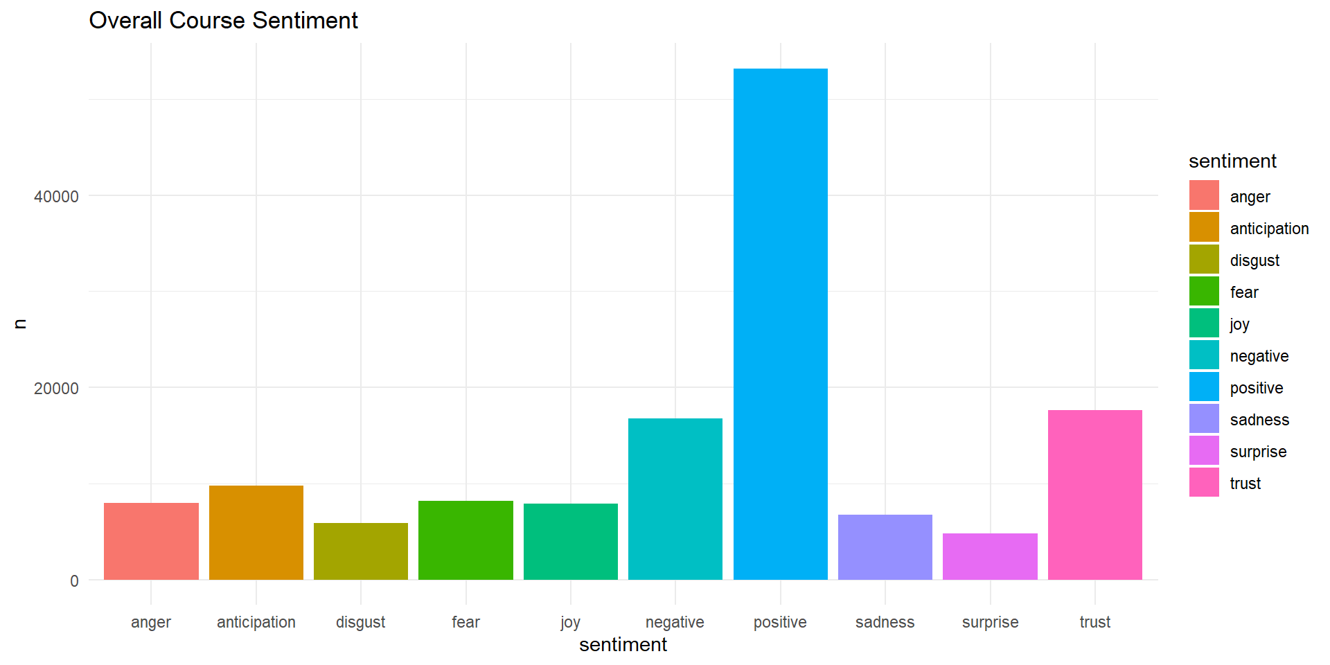
# A tibble: 10 × 2
   sentiment        n
   <chr>        <int>
 1 anger         8000
 2 anticipation  9756
 3 disgust       5913
 4 fear          8173
 5 joy           7894
 6 negative     16783
 7 positive     53188
 8 sadness       6743
 9 surprise      4814
10 trust        17595
Visualizing Sentiment
- Effective for quickly visualizing sentiment counts in a text
- Can be used with other variables to answer questions like: What weeks had the highest frustration within a course?
- We use
ggplot2to bring these numbers to life
- Visualize the most common positive words in a program
- R can generate these easily using packages like
wordcloud - Word clouds are highly favored by leadership and executive summaries but should be used with care and intention
Critical Limitations
Despite these benefits, dictionaries can’t “read:”
- Sarcasm: “Oh great, another 50-page reading” (R thinks “great” is positive).
- Negation: “Not helpful” (R sees “helpful” and sees it as positive).
- Context: “The exam was sick”.
Ethical Considerations
- Privacy: Anonymize student text before analysis. Remove names and ID numbers.
- Bias: Lexicons are built by humans and may carry cultural or historical biases.
- A Human Touch: Never use sentiment scores as the only reason to change a grade or evaluate a teacher. Useful as a conversation starter but not the end-all.
❓Discussion
Where could you see dictionary-based sentiment analysis coming in handy in your work?
What are some ways that your college or university may read too much into sentiment analysis for their own evaluation and policy development?
Acknowledgements

This work was supported by the National Science Foundation grants DRL-2025090 and DRL-2321128 (ECR:BCSER). Any opinions, findings, and conclusions expressed in this material are those of the authors and do not necessarily reflect the views of the National Science Foundation.